
Color Visualization of 2D Segmentations
Christoph Dalitz, Tobias Bolten and Oliver Christen
Institute for Pattern Recognition, Niederrhein University of Applied Sciences, Reinarzstr. 49, Krefeld, Germany
Keywords:
Visualization of Spatial Data, Area Voronoi Diagram, Graph Coloring, Color Metrics.
Abstract:
This paper deals with the problem of coloring a two-dimensional segmentation result in such a way that each
segment has a different color with the constraint that adjacent segments have sufficiently distinct colors to be
easily distinguishable by a human viewer. Our solution for this problem is based on a balanced coloring of the
neighborhood graph built from the area Voronoi diagram. The balanced coloring with only a limited number
of colors is subsequently modified to assign each segment a unique color. For picking the initial palette of
evenly distributed colors, we propose a method that is based on the physical analogy of energy minimization
in a Wigner crystal. To make the energy formula applicable to arbitrary color spaces and distance measures,
we give generalized definitions for the center and radius of a color space with an arbitrary distance metric.
The individual steps of our coloring algorithm have been evaluated on the PRIMA dataset.
1 INTRODUCTION
Segmentations of images are typically visualized as
color images, in such a way that pixels belonging to
the same segment have the same color, while pixels
belonging to different segments have different colors
(Saund et al., 2009) (Shafait et al., 2006). When the
segmentation has to be checked or corrected by a hu-
man observer, it is however not sufficient to assign
different colors to different segments, because adja-
cent segments are hard to distinguish when their col-
ors are too similar. This applies in particular to docu-
ment image segmentation, in which the segments rep-
resenting text lines, paragraphs, words, characters, or
similar are embedded in white background. Hard to
distinguish neighboring segments are both a problem
when looking for segmentation errors by visual in-
spection, as well as in the process of creating ground
truth data for segmentation evaluation studies or train-
ing purposes.
Ideally, the chosen coloring would satisfy a gener-
alized graph coloring problem:
Given a neighborhood graph of n segments,
n colors c
1
,...,c
n
, and a distance metric
d(c
i
,c
j
) on the colors, find a node color-
ing that maximizes the minimum distance be-
tween adjacent colors.
Some ordinary graph coloring problems are special
cases of this problem: the “equitable coloring prob-
lem” (Pemmaraju et al., 2003), e.g., is the special case
of only k different colors evenly distributed among the
c
1
,...,c
n
, and d being the trivial metric. In the gen-
eral case of a nontrivial metric, this is a difficult op-
timization problem that presumably cannot be solved
in polynomial time.
Our goal in the present paper is therefore more
modest: we only propose algorithms for selecting and
assigning colors in such a way that the minimum dis-
tance between adjacent colors is “not too small”. Our
approach consists of two steps: first the neighborhood
graph is colored with only a small number of colors.
Each of these colors is then considered as the center
of a color cluster, whose colors are distributed among
the nodes belonging to the center color.
2 THE NEIGHBORHOOD GRAPH
There are different definitions of segment “neighbor-
hood”, some based on geometric distance and others
based on adjacency. In our case, we are not interested
in the nearest neighbors of a segment, but in all adja-
cent segments. It is thus natural to define the neigh-
borhood graph as the dual graph of the area Voronoi
diagram generated by the segments.
2.1 The Area Voronoi Diagram
For a set of two dimensional points P = {p
1
,..., p
n
},
the ordinary (or point) Voronoi diagram is a tessel-
567
Dalitz C., Bolten T. and Christen O..
Color Visualization of 2D Segmentations.
DOI: 10.5220/0004184905670572
In Proceedings of the International Conference on Computer Graphics Theory and Applications and International Conference on Information
Visualization Theory and Applications (IVAPP-2013), pages 567-572
ISBN: 978-989-8565-46-4
Copyright
c
2013 SCITEPRESS (Science and Technology Publications, Lda.)

Figure 1: A point Voronoi diagram (left) and an area
Voronoi diagram of three segments (right).
lation of the plane into disjoint cells such that the
Voronoi cell of point p
i
is given by
V(p
i
) = {p : kp− p
i
k ≤ kp−p
j
k for all j 6= i}
where kp −qk denotes the Euclidean distance be-
tween p and q. In other words, every point in V(p
i
)
is closer to p
i
than to each other point in P. Fig. 1
shows the resulting Voronoi cells for a sample set
of six points. The Delaunay graph associated to a
Voronoi diagram has a node for each Voronoi cell and
edges between neighboring cells.
The area Voronoi diagram is a generalization of
the ordinary Voronoi diagram in such a way that the
tessellation is not generated by points, but by non
overlapping objects S = {s
1
,...,s
n
}. Every point in
the Voronoi cell V(s
i
) is then closer to object s
i
than
to any other object:
V(s
i
) = {p : min
q∈s
i
kp −qk≤ min
q∈s
j
kp −qk for all j 6= i}
The right figure in Fig. 1 shows the area Voronoi cell
boundaries for an example of three objects. In our
application case, the objects are the segments of the
segmentation. The sought neighborhood graph then
corresponds to the area Voronoi diagram. Let us call
this neighborhood graph the area Delaunay graph.
2.2 Computing the Area Delaunay
Graph
As the area Voronoi diagram can be useful for
bottom-up page segmentation, a number of methods
have been suggested for its computation (Arcelli and
di Baja, 1986) (Lu and Tan, 2005) (K. Kise, 1998).
For instance, it can be computed exactly with a re-
gion growing approach, which can either be done di-
rectly on the image with pixel labeling, or on some
representation of the segment contours. To reduce
the runtime, Kise et al. suggested to compute the
area Voronoi diagram approximately by first comput-
ing the point Voronoi diagram from contour sample
points and then merging cells belonging to the same
segment (K. Kise, 1998).
When only the area Delaunay graph is of inter-
est and the exact shape of the Voronoi cells does
not matter, the contour sample points can be used
to directly compute a point Delaunay triangulation.
The area Delaunay graph is then obtained by merging
nodes belonging to the same segment. We have cho-
sen this approach because it can be done efficiently
in O(nlogn) time for n points (Devillers, 2002). For
a typical document layout, the sample points contain
several collinear points which result in degenerate tri-
angles that incorrectly have edges between non adja-
cent points. It is therefore necessary to clean up these
triangles after computing the triangulation.
Concerning the sampling rate for the contour
points, the experiments described in Sec. 4.1 have
shown that taking between 20% and 30% of the con-
tour points yields a reasonable compromise between
accuracy and speed.
3 COLORING THE GRAPH
Our coloring algorithm for the neighborhood graph is
a two step approach: first the graph is colored with a
small number k of colors; then this coloring is modi-
fied so that every node obtains a differentcolor. In two
subsections, we propose algorithms for the following
problems: (a) how to choose the initial k colors and
the final full set of n colors, and (b) how to do the
initial k-coloring and modify it to an n-coloring.
3.1 Color Selection
The problem of color palette selection is usually con-
sidered under the optimization criterion of a best
match between the palette and given images. An
interesting exception is Moijsilovi´c and Soljanin’s
scheme for picking a color palette from a spiral lat-
tice in the CIE L*a*b* color space (Mojsilovic and
Soljanin, 2001). The resulting colors however depend
on a number of input parameters and it is not even
clear which input parameters lead to a given number
n of valid colors in RGB space, nor have they pro-
posed criteria for “good” parameter choices.
In our situation, we seek k colors c
1
,...,c
k
that
are “most different” from each other. Each color c
i
is a vector of three values representing red, green and
blue. Defining a color distance measure that mod-
els visual perception is a very difficult problem, and a
wide variety of distance measures d(c
i
,c
j
) have been
proposed. The best known are the Euclidean distance
in RGB space d
RGB
or the CIE L*a*b* color distance
d
Lab
:
d
RGB
(c
i
,c
j
) = kc
i
−c
j
k
d
Lab
(c
i
,c
j
) =
(L(c
i
) −L(c
j
))
2
+ (a(c
i
) −a(c
j
))
2
IVAPP2013-InternationalConferenceonInformationVisualizationTheoryandApplications
568

+(b(c
i
) −b(c
j
))
2
1/2
(1)
More sophisticated distance measures include the
CIE94 and the HCL color distance (Sarifuddin and
Missaoui, 2005), or the DIN99 distance (Deutsches
Institut f¨ur Normung, 2001).
Concerning the “optimality” criterion for the color
palette, let us first observe that in an Euclidean space,
an optimal equidistant distribution is taken on by elec-
trons repelling each other, a configuration also known
as Wigner or Coulomb crystal (Rafac et al., 1991).
The equilibrium distribution of these minimizes the
electric potential energy
ϕ(c
1
,...,c
k
) =
∑
i> j
e
2
kc
i
−c
j
k
+
∑
i
γkc
i
k
2
(2)
where e denotes the electric charge of the electrons
and γ is the strength of a harmonic attractor in the
center. It is thus natural to define as a criterion for
the optimal color palette that it minimizes (2) with
the Euclidean distance kc
i
−c
j
k replaced with a color
distance measure d(c
i
,c
j
). As we cannot use the color
white w (reserved for the image background) and ad-
ditionally would like to keep the color black b for
noise left over from an incomplete segmentation, we
add the “potential energy” stemming from these two
points to (2). This means that we seek to minimize
ϕ(c
1
,...,c
k
) =
∑
i> j
1
d(c
i
,c
j
)
+
∑
i
γ
d(c
i
,µ)
2
+
∑
i
α
d(c
i
,w)
+
∑
i
β
d(c
i
,b)
(3)
where each color c = (c
r
,c
g
,c
b
) is subject to the con-
straint 0 ≤ c
r
,c
g
,c
b
≤ 255, and µ is the center of the
color space (see Sec. 4.2 for a precise definition of this
center). The constants α and β have been introduced
for convenience so that it is possible to optionally en-
force a smaller or larger distance of the colors from
black or white.
In Sec. 4.2, the resulting color distribution for dif-
ferent color metrics and k = 6 (the minimum num-
ber of colors for the coloring algorithm described
in Sec. 3.2) is given. Interestingly, the best results
are not obtained with the more sophisticated distance
measures, but with the simple Euclidean distance in
the RGB space.
For the final full set of n different colors, we con-
sider each of the initial k colors c
1
,...,c
k
to be the
core of a “color cluster” of n/k colors. We subse-
quently add colors one-by-one to a cluster around c
i
,
such that each added color fulfils two conditions:
• on the discrete RGB color grid, it is the neighbor
to one of the colors that are already in the clusters
• among all possible new neighbors, the neighbor c
with the closest distance to the color center c
i
is
chosen.
3.2 Balanced Coloring and its
Modification
As the area Delaunay graph is planar, it can be col-
ored in linear time, e.g. with the 6-COLOR algorithm
by Matula et al. (Matula et al., 1980). This algorithm,
however, does not produce a balanced coloring, be-
cause among the colors not yet used in a node neigh-
borhood it always picks the “smallest” color. We have
replaced this color selection step with a simple heuris-
tic: instead of the smallest color, we select the color
that has been used least frequently so far. This simple
rule lead to an equitable coloring in almost all of our
experiments described in Sec. 4.3.
To modify the initial balanced k-coloring into a
complete n-coloring, the n/k colors of each color
cluster need to be distributed among the nodes as-
signed to the respective color cluster. To this end, we
have implemented three different methods, which all
traverse the graph in a breadth-first search. They dif-
fer in the way a color for a node belonging to color
cluster C
i
is chosen, based on the colors already as-
signed to its neighbors:
a) random method: select a random yet unused color
from C
i
b) maxdist method: select the yet unused color from
C
i
with the greatest distance to the neighbor node
colors
c) coredist method: select the yet unused color from
C
i
with a distance to its closest neighbor node
color similar to the distance between the color
cluster cores
In our experiments (see Sec. 4.4), the random and
the coredist method were comparable and better than
the maxdist method. For most practical purposes, the
simple random method will thus be a sufficient solu-
tion, that is both easy to implement and efficient.
4 EXPERIMENTS AND RESULTS
We did a number of experiments to evaluate the indi-
vidual steps of our algorithm, which we have imple-
mented in C++ within the Gamera framework for doc-
ument analysis and recognition
1
. As document test
images, we used the PRIMA dataset (Antonacopou-
los et al., 2009) which, at the time of our experiments,
1
http://gamera.sf.net/
ColorVisualizationof2DSegmentations
569

[sec]
runtime
rate
error
10 30 50 70 90
0.0
2.0
4.0
6.0
runtime
error
0.06
0.04
0.02
0.00
contour sampling rate [%]
Figure 2: Effect of the contour sampling rate on the edge
error rate and on the runtime.
consisted of the 55 test images from the page segmen-
tation competition of the two ICDAR conferences in
2007 and 2009. As the segments to be colored, we
did not consider the segments marked in the ground
truth data, but the connected black components, be-
cause these were much more segments (about 5200
per image).
4.1 Sampling Rate for the Delaunay
Graph
For different contour sampling rates, we have mea-
sured the number of edges in the resulting Delau-
nay graph that differ from a reference graph with a
100% sampling rate. The average results over all im-
ages, with the runtimes measured on an Intel Core2
1.66GHz processor,are shown in Fig. 2. It can be seen
that a sampling rate between 20% and 30% yields an
error rate already below 1.5%, thereby setting a rea-
sonable compromise between accuracy and speed.
4.2 Optimal Initial k Colors
To numerically compute the color configuration that
minimizes Eq. (3), we have used the Monte Carlo
algorithm described by Rafac et al. in (Rafac et al.,
1991). It simply consists in moving downhill from
N randomly chosen starting points and picking the
global minimum from these local minima. We chose
N = 1000. When applying Eq. (3), the question arises
how to choose the attracting strength γ, which is re-
lated to the radius r of the Coulomb cluster. For an
unconstrained Euclidean space, (Rafac et al., 1991)
gives the relation
2r ≈ k
0.4687
(2γ)
−1/3
(4)
Solving for γ and setting 2r =
√
3·255 yields the re-
lation how to increase γ with k in the Euclidean RGB
space. The resulting minimum energy configurations
for α = β = 1 for different values of k are displayed
in Fig. 3.
Generalizing Eqs. (3) and (4) to an arbitrary color
space first requires an appropriate definition of the
center color µ and the radius r of the color space.
A generalized definition of the arithmetic mean µ of
x
1
,...,x
N
can be derived from its property to mini-
mize
∑
i
kx
i
−µk
2
. We thus define the center color µ
and the radius r of a color space with color distance d
as
µ = argmin
m
∑
c
d(c,m) (5)
r = max
c
d(c,µ) (6)
where c runs over all possible RGB colors. The
numerical values resulting from this definition are
listed in Tbl. 1 for six different distance metrics:
the Euclidean distance in RGB and L*a*b* space,
the DIN99 distance (Deutsches Institut f¨ur Normung,
2001), the CIE94 and HCL distance (Sarifuddin and
Missaoui, 2005), and the cylindrical distance in HSV
space (Ikonomakis and Plataniotis, 1999).
Using the values from Tbl. 1 and with α = β = 1,
we have determined the minimum energy choice of
k = 6 colors. This is a natural choice for k, because
it is the minimum number of colors required by the
graph coloring algorithm 6-COLOR. Moreover, in
this case the energy minimum with respect to the Eu-
clidean distance in RGB is already known (six colors
in the corners of the RGB cube), which provides a
nice benchmark against which we can compare other
0 0 127
0 255 127
127 127 0
127 127 255
255 0 0
255 0 127
255 0 255
255 255 0
255 255 127
0 255 255
0 0 255
0 255 0
Blue
Red
Green
(a) k = 12
0 0 127
255 0 0
255 0 255
255 127 0
255 255 0
255 255 127
0 255 255
127 255 255
255 127 255
0 0 255
0 127 255
127 255 0
127 127 127
0 255 0
0 127 0
127 0 0
255 0 127
127 0 255
0 255 127
Blue
Red
Green
(b) k = 19
0 0 127
0 127 0
0 255 0
0 255 127
127 0 127
127 0 255
127 255 0
128 128 0
255 0 0
255 0 127
255 0 255
255 127 0
255 255 0
255 255 127
0 255 255
127 255 255
0 127 255
0 0 255
127 255 128
127 0 0
128 127 255
255 127 255
Blue
Green
Red
(c) k = 22
Figure 3: Minimum energy configurations for k colors in the Euclidean RGB space.
IVAPP2013-InternationalConferenceonInformationVisualizationTheoryandApplications
570
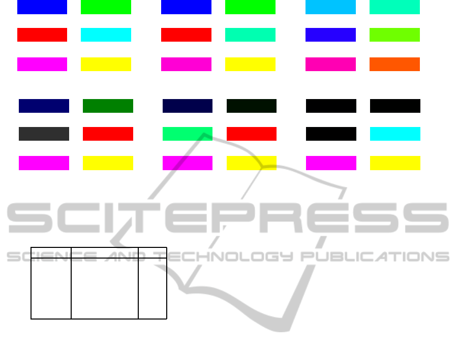
(000,255,000)(000,000,255)
(000,255,255)(255,000,000)
(255,255,000)(255,000,255)
(a) RGB
(000,255,000)(000,000,255)
(255,255,000)(255,000,213)
(255,000,000) (000,255,177)
(b) L*a*b*
(000,195,255)
(038,000,255) (111,255,000)
(255,000,179) (255,87,000)
(000,255,186)
(c) HCL
(255,255,000)(255,000,255)
(000,000,111) (000,128,000)
(047,047,047) (255,000,000)
(d) CIE94
(255,255,000)
(000,000,075) (000,017,000)
(000,255,112) (255,000,000)
(255,000,255)
(e) DIN99
(000,001,000)(000,000,001)
(000,255,255)(001,000,000)
(255,255,000)(255,000,255)
(f) HSV
Figure 4: The color distributions minimizing Eq. (3) with respect to different color distance metrics.
Table 1: RGB values of center and radius of different color
space according to Eqs. (5) and (6).
µ r
RGB (127,127,127) 220
L*a*b* (135,130,126) 142
HCL (210,209,209) 311
CIE94 (133,137,107) 83
DIN99 (128,124,120) 82
HSV (194,194,194) 1.25
color distance metrics. Fig. 4 shows the results for the
six different distance metrics.
Both the HCL and L*a*b* distance result in a
poorer distribution than the RGB distance, because
both include two similar green hues. Interestingly, the
same HCL and L*a*b* results are obtained when the
RGB result is used as a starting point for the mini-
mization algorithm: both distance metrics make the
distribution worse. Even though the CIE94 distance
results in six visually different colors, one of them is
almost black, despite the repelling potential from the
β-term in Eq. (3). The same applies to the DIN99 dis-
tance which even leads to two colors that are almost
black. For the cylindrical HSV distance, we obtain
even three almost black colors, but this is due to a
fundamental shortcoming of this distance measure in
case of colors that have a low intensity, but a high sat-
uration because one of the primary colors is zero.
Our experiments thus provide a justification for
the intuitive approach to select colors in the cor-
ners of the RGB cube, even though this includes the
somewhat similar colors green (0,255,0) and cyan
(0,255,255). Finding a color distance measure and an
optimization criterion that perceptually improves this
distribution is an interesting area of further research.
4.3 Balance of the Initial k-coloring
A coloring is equitable, when the color counts do not
differ by more than one (Pemmaraju et al., 2003). Our
balanced variant of the 6-COLOR algorithm pro-
duced indeed equitable colorings for 51 of the 55 test
images. In each of the remaining four images, there
was one color count difference of two and the other
counts differed not more than one. This shows that
the simple heuristic color selection rule indeed results
in a balanced coloring.
4.4 Quality of the Final n-coloring
To compare the quality of the three color distribu-
tion methods described in Sec. 3.2, we have measured
both the minimum and the average RGB distance be-
tween neighboring node colors. Tbl. 2 lists the av-
eraged results over the N = 55 test images. Both
the minimum and average distances decrease with the
number k of initial colors. This shows that our ap-
proach of building color clusters around few initial
colors is an improvement over the naive approach
of picking n evenly distributed initial colors, which
would be the extreme case k = n.
All three methods for modifying the k-coloring
into an n-coloring lead to similar mean and minimum
color distances between neighboring nodes. The sim-
ple maxdist method, which always picks the most far
away color among all free colors from a color cluster,
leads to the largest distance. Even though the ran-
dom method leads to smaller distances, its runtime
is only linear in the number of nodes, while the run-
times other two methods are quadratic in the number
of nodes. The random assignment of colors from a
ColorVisualizationof2DSegmentations
571

Table 2: Mean and minimum RGB color distance between
neighboring nodes for the three color distribution methods
and different numbers k of core colors, averaged over all
images from the PRIMA dataset.
method mean dist min dist
k = 6 maxdist 325.6 239.3
random 325.1 234.6
coredist 325.3 235.4
k = 16 maxdist 259.8 120.0
random 259.0 115.0
coredist 259.6 115.4
k = 26 maxdist 233.8 77.4
random 233.3 73.1
coredist 233.6 73.9
cluster to its nodes will therefore often be a sufficient
and reasonable approach in practice.
5 CONCLUSIONS
The methods proposed in this paper provide a practi-
cal solution for using colors as segmentation labels in
such a way that the segmentation is easily visible in
the resulting color image for a human observer.
Nevertheless, there remain two interesting areas of
further research. One consists in finding better ways
for selecting the initial k colors, both with respect to
the optimization criterion Eq. (3) and to an appropri-
ate color distance measure. As the latter problem of
defining a perceptual color distance is a very diffi-
cult problem still waiting for satisfactory solutions,
it might alternatively be more promising to perform
psychological experiments for directly selecting the k
perceptually “most different” colors. The other open
problem is the more fundamental algorithmic ques-
tion whether there is an efficient exact or approximate
solution for the generalized graph coloring problem
stated in the introduction.
REFERENCES
Antonacopoulos, A., Bridson, D., Papadopoulos, C., and
Pletschacher, S. (2009). A realistic dataset for per-
formance evaluation of document layout analysis. In
International Conference on Document Analysis and
Recognition (ICDAR), pages 296–300.
Arcelli, C. and di Baja, G. S. (1986). Computing voronoi
diagrams in digital pictures. Pattern Recognition Let-
ters, 4:383–389.
Deutsches Institut f¨ur Normung (2001). Farbmetrische Bes-
timmung von Farbabst¨anden bei K¨orperfarben nach
der DIN99-Formel. DIN 6176.
Devillers, O. (2002). The delaunay hierarchy. International
Journal of Foundations of Computer Science, 13:163–
180.
Ikonomakis, N. and Plataniotis, K. (1999). A region-based
color image segmentation scheme. In Visual Commu-
nications and Image Processing (VCIP), pages 1201–
1209.
K. Kise, A. Sato, M. I. (1998). Segmentation of page images
using the area voronoi diagram. Computer Vision and
Image Understanding, 70:370–382.
Lu, Y. and Tan, C. (2005). Constructing area voronoi di-
agram in document images. In International Con-
ference on Document Analysis and Recognition (IC-
DAR), pages 342–346.
Matula, D., Shiloach, Y., and Tarjan, R. (1980). Two linear-
time algorithms for five-coloring a planar graph. Tech-
nical Report STAN-CS-80-830, Stanford University.
Mojsilovic, A. and Soljanin, E. (2001). Color quantization
and processing by fibonacci lattices. IEEE Transac-
tions on Image Processing, 10:1712–1725.
Pemmaraju, S., Nakprasit, K., and Kostochka, A. (2003).
Equitable colorings with constant number of colors.
In ACM-SIAM Symposium on Discrete Algorithms
(SODA), pages 458–459.
Rafac, R., Schiffer, J., Hangst, J., Dubin, D., and Wales, D.
(1991). Stable configurations of confined cold ionic
systems. Proc. Ntl. Acad. Sci. USA, 88:483–486.
Sarifuddin, M. and Missaoui, R. (2005). A new perceptually
uniform color space with associated color similarity
measure for content-based image and video retrieval.
In ACM SIGIR Workshop on Multimedia Information
Retrieval, pages 1–8.
Saund, E., Ling, J., and Sarkar, P. (2009). Pixlabeler: User
interface for pixel-level labeling of elements in docu-
ment images. In International Conference on Docu-
ment Analysis and Recognition (ICDAR), pages 646–
650.
Shafait, F., Keysers, D., and Breuel, T. (2006). Pixel-
accurate representation and evaluation of page seg-
mentation in document images. In International Con-
ference on Pattern Recognition (ICPR), pages 872–
875.
IVAPP2013-InternationalConferenceonInformationVisualizationTheoryandApplications
572
