
Medical Volume Segmentation based on Level Sets of Probabilities
Yugang Liu
1
and Yizhou Yu
2
1
Department of Computer Science and Engineering,
University of Electronic Science and Technology of China, Chengdu, China
2
University of Illinois at Urbana-Champaign, Illinois, U.S.A.
Keywords:
Medial Image Segmentation, Level Set Method, Discriminative Probabilistic Classifier.
Abstract:
In this paper, we present a robust and accurate method for biomedical image segmentation using level sets of
probabilities. The level set method is a popular technique in biomedical image segmentation. Our method
integrates a probabilistic classifier with the level set method, making the level set method less vulnerable to
local minima. Given the local attributes within a neighborhood of a voxel, this classifier outputs an estimated
likelihood of the voxel being part of an object of interest. Our method obtains a posterior probabilistic mask
of the object of interest according to such estimated likelihoods, an edge field and a smoothness prior. We
further alternate classifier training and the level set method to improve the performance of both. We have
successfully applied our method to the segmentation of various organs and tissues in the Visible Human
dataset. Experiments and comparisons demonstrate our method can accurately extract volumetric objects
of interest, and outperforms traditional levelset-based segmentation algorithms.
1 INTRODUCTION
The growing size and number of these medical images
have necessitated the use of computers to facilitate
processing and analysis. In particular, computer algo-
rithms for the delineation of anatomical structure and
other regions of interest are becoming increasingly
important in assisting and automating specific radi-
ological tasks (Pham et al., 2000). Three-dimensional
segmentation of biomedical volumetric image data, a
foundation of high-level medical image analysis, has
important significance in biomedical engineering.
The level set method (LSM) is a popular tech-
nique in biomedical image segmentation. This is
due to many reasons. LSM represents the segmenta-
tion boundary in an implicit and parameter-free way,
which is convenient for checking whether points be-
long to the interior of the segmented region. The im-
plicit representation is also particularly convenient for
evolving the topology of the segmentation boundary
during a solution process. Furthermore, LSM can be
used to define a generic optimization framework. All
sorts of criteria judging the quality of a segmentation
can be integrated into this framework as priors. Thus
solving this generic optimization can be cast as solv-
ing the PDE of the level set method.
Nevertheless, a serious limitation of many exist-
ing level set algorithms for image segmentation is that
the final result is very sensitive to the location of the
initialization. This is because the above optimization
typically has many local minima to trap level set evo-
lution, which is driven by forces computed from local
image data in the vicinity of the zero level set.
In this paper, we present an interactive volume im-
age segmentation technique that overcomes this limi-
tation. This technique generalizes the 2D image seg-
mentation algorithm presented in (Liu and Yu, 2012),
which integrates a discriminative classifier with the
level set method. The classifier performs pixelwise
classification over the entire image domain and feeds
information garnered during this process to the level
set method, which thus gains a more “global” under-
standing regarding which local image regions likely
belong to an object of interest.
However, generalizing the 2D segmentation algo-
rithm in (Liu and Yu, 2012) to volume images im-
poses a few challenges. First, volume images typi-
cally have less color and texture variations. It is un-
clear how to define effective volume texture descrip-
tors and volume edges which provide important infor-
mation to the classifier as well as the level set method.
Second, the number of voxels in a volume image is
much larger than the number of pixels in a 2D image.
It is unclear how to perform voxelwise classification
in a reasonably efficient way while still guarantee a
high classification accuracy.
387
Liu Y. and Yu Y..
Medical Volume Segmentation based on Level Sets of Probabilities.
DOI: 10.5220/0004185903870394
In Proceedings of the International Conference on Computer Vision Theory and Applications (VISAPP-2013), pages 387-394
ISBN: 978-989-8565-47-1
Copyright
c
2013 SCITEPRESS (Science and Technology Publications, Lda.)

In summary, the contributions of this paper are as
follows.
• We generalize the weakly supervised levelset-
based 2D image segmentation framework in (Liu
and Yu, 2012) to three-dimensional volume im-
ages. Experiments and comparisons indicate this
generalized algorithm can accurately extract vol-
umetric objects of interest without the assistance
of a shape prior, and outperforms the graphcut al-
gorithm and traditional levelset-based algorithms
on volume images.
• In our generalized algorithm, we adopt a boosted
logistic classifier as the probabilistic classifier in-
tegrated with the level set method. In comparison
with other boosted classifiers, this one can be eval-
uated efficiently on new testing data while main-
taining comparable classification accuracy.
• We also extend 2D edge and texture feature ex-
traction to 3D volume images.
2 BACKGROUND AND RELATED
WORK
In this section we review previous segmentation tech-
niques and focus on level set methods for biomedical
images. The majority of previous work on levelset
based image segmentation is unsupervised except for
(Paragios and Deriche, 1999; Liu and Yu, 2012),
where a user can provide hints by drawing boxes or
a convex hull over the foreground object. In compar-
ison with the interactive segmentation method in this
paper, the work in (Paragios and Deriche, 1999) only
adopts a relatively simple statistical model and does
not consider distant interactions with edge pixels. As
a result, region boundaries are often trapped in local
minima, and do not snap to true object boundaries.
A state-of-the-art levelset based technique for inter-
active segmentation of 2D natural images has been
presented in (Liu and Yu, 2012), where the level set
method is integrated with a discriminative probabilis-
tic classifier and carefully designed features are used
for differentiating textures. In this paper, we gener-
alize the method in (Liu and Yu, 2012) to volumetric
biomedical images.
A method for segmenting thin structures has been
presented in (Holtzman-Gazit et al., 2006), which in-
tegrates edge information with the minimal variance
criterion for segmented regions. However, the mini-
mal variance criterion is a simple classifier that can-
not cope with complex textures in medical images.
Because of its unsupervised nature, the presented re-
sults in this paper do not have very accurate object
boundaries. A method for segmenting brain tumor
in MRI images has been presented in (Cobzas et al.,
2007). However, this approach has to learn a statisti-
cal model for tumor and normal tissue using manually
segmented data. A method for segmenting medical
images using hybrid discriminative/generativemodels
has been presented in (Tu et al., 2008). This method
integrates a discriminative classifier with a genera-
tive shape model. Region boundary evolution based
on this hybrid model is performed using the level set
method. However, this approach is still a region-
growing method and cannot handle objects with a
complex topology very well.
3 OVERVIEW
The key idea of level sets of probabilities is to inte-
grate a probabilistic voxel classifier with the level set
method, making the level set method less vulnerable
to local minima. Given the attributes within a neigh-
borhood of a voxel, this classifier outputs an estimated
likelihood of the voxel being part of an object of inter-
est. Our goal is to obtain a voxelwise posterior prob-
ability based on this estimated likelihood and certain
prior models of the object of interest. To integrate
the classifier with the level set method, we attempt to
make a transformed version of the level set function,
Φ(x,t), achieve an increasingly better approximation
of a posterior probabilistic mask of the object of inter-
est over time. Since probabilities fall into [0,1] while
the values of our level set function belong to [−1, 1]
with positivevalues falling outside the zero levelset, a
voxelwise probabilistic mask needs to be transformed
as follows to become a level set function:
Φ(x) = −2(P(l(x) = 1|I) − 0.5), (1)
where l(x) denotes the label of voxel x, and P(l(x) =
1|I) represents the posterior probability of voxel x be-
ing part of the object of interest. Generally speaking,
there are few necessary conditions if any that a level
set function has to satisfy except that Lipschitz conti-
nuity is a desired property for sampling and numerical
approximation (Osher and Fedkiw, 2003). Since the
probability values at two adjacent voxels can at most
differby one, our levelset function by default has Lip-
schitz continuity. In practice, we also apply low-pass
filtering to the latest level set function at the end of
each time step to make it smoother.
Since our method belongs to supervised level set
methods, it requires a small amount of user interac-
tion. The user can simply draw 3D boxes around local
regions in the object of interest as well as in the back-
ground (Fig. 1(b)). Given initial user-supplied boxes,
VISAPP2013-InternationalConferenceonComputerVisionTheoryandApplications
388
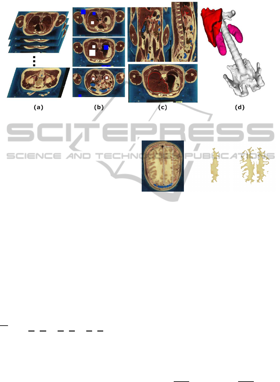
Figure 1: The pipeline of our method. (a) Biomedical volumetric image data, (b) initial user-drawn regions (white for object,
blue for background), (c) the final segmentation result (red curve is the zero level set), (d) 3D visualization (white for spine,
pink for kidneys, red for liver).
a probabilistic voxel classifier can be trained. And
the level set function is initialized according to voxel-
wise likelihoods estimated by the probabilistic classi-
fier. Once initialized, we run the level set method until
it converges to obtain a mask of the object of interest.
Note that we can alternate classifier training and the
level set method to improve the performance of both.
Fig. 2 shows a comparison of the results that can
be achieved with traditional level set methods and our
new method. Obviously, a traditional level set method
can easily return a local minimum as a solution, which
omits the white matter on the left cerebral hemisphere
in the image. In contrast, all the white matter can be
extracted with our algorithm.
4 LEVEL SETS OF
PROBABILITIES
Our level set method tracks the evolution of the
front by numerically solving the following differen-
tial equation and extracting the zero level set of the
solution:
∂Φ
∂t
= −
α· R(x,t)
| {z }
classifier
+β·B(x,t)
| {z }
edge field
+γ·C(x,t)
| {z }
curvature
k∇Φk,
(2)
where x denotes voxel coordinates in the image and
t denotes the time of advection. In (2), the evolution
of the zero level set is driven by three force terms, the
classifier force, edge field force, and curvature force,
which will be briefly discussed below as they are
adapted from the force terms in (Liu and Yu, 2012).
(a) (b) (c)
Figure 2: Comparison of segmented white matter in a med-
ical image. (a) Initial user-drawn white rectangle, (b) seg-
mentation result from a traditional level set method, (c) seg-
mentation result from our revised level set method.
The equation in (2) can be efficiently solved using
the narrow band method in (Sethian, 1999; Osher and
Fedkiw, 2003) and the fast local level set method in
(Peng et al., 1999).
• Classifier Force. We define the following energy
term E
R
to measure the degree of inconsistency be-
tween global posterior probabilities and local likeli-
hoods returned by the voxel classifier:
E
R
=
ZZZ
I
Φ(x) − Φ
0
(x)
2
dx, (3)
where Φ
0
(x) = −2(P(l(x) = 1|N(x)) − 0.5), where
P(l(x) = 1|N(x)) denotes the likelihood of voxel x
being part of the object of interest according to the
probabilistic classifier, which only gathers evidences
available from a local neighborhood N(x). By taking
the derivative of (3) with respect to the level set pass-
ing through x, we obtain the following force term that
reduces the energy in (3):
R(x)
∇Φ
k∇Φk
=
Φ(x) − Φ
0
(x)
∇Φ
k∇Φk
, (4)
MedicalVolumeSegmentationbasedonLevelSetsofProbabilities
389

where
∇Φ
k∇Φk
represents the unit outward normal vector
of the zero level set.
• Edge Field Force. A second goal is to make the zero
level set snap to salient edges in the volume image be-
cause salient edges are likely to lie on the boundary
surface of the object of interest. This is achieved with
an unsigned distance transform of salient edge vox-
els, Ψ(x). We adopt the following energy term E
B
to
measure the overall proximity between the zero level
set and the set of salient edges:
E
B
(Ω) =
ZZ
Ω
Ψ(x(u,v))kΩ
u
× Ω
v
kdudv, (5)
where Ω(u, v) is a 2D parametrization of the zero
level set, and u ∈ [0,1], v ∈ [0,1], respectively. x :
Ω → I is a mapping from parametric coordinates to
3D image coordinates.
With such an energy term in mind, we define the
second force term for boundary localization as fol-
lows:
B(x)
∇Φ
k∇Φk
= −
∇Ψ(x) ·
∇Φ(x)
k∇Φ(x)k
∇Φ
k∇Φk
, (6)
which tries to move the zero level set towards salient
edges by following the negative gradient of the edge
field.
• Curvature Force. The curvature force is a standard
term in level set methods. Our curvature force tries to
provide a tradeoff between boundary smoothness and
boundary faithfulness. That means in the vicinity of
edges, boundary localization is still a more important
goal than boundary smoothness. But in the absence
of edges, boundary smoothness serves as an effective
prior to determine the shape and position of the lo-
cal object boundary. We define the curvature force as
follows:
C(x)
∇Φ
k∇Φk
= −(µκ(x) + (1 − µ)Ψ(x)κ(x))
∇Φ
k∇Φk
,
(7)
where κ(x) denotes the mean curvature of the level set
surface passing through x, and 0 ≤ µ ≤ 1. The second
term in (7) modulates curvature with the edge field to
weaken the curvature force in the vicinity of edges.
Nevertheless, the first term guarantees that the curva-
ture force does not disappear completely as long as µ
remains positive. A formula for the mean curvature
of the zero level set in a three-dimensional space can
be found in (Osher and Fedkiw, 2003),
The evolution of the zero level set driven by the
force in (2) is illustrated in Fig. 3. The initial zero
level set is fragmented because of the noisy voxelwise
likelihoods from the classifier. Note that although be-
ing fragmented, these contours spread over the en-
tire object, making the level set method less likely
to be stuck in local minima. These initial contours
are evolved by the level set method. They gradually
merge with each other and also move toward true ob-
ject boundaries to improve their localization and spa-
tial coherence. Thus, our segmentation algorithm can
also be viewed as an advanced version of region-split-
and-merge algorithms.
4.1 Discriminative Probabilistic
Classifier
Our level set method relies on the accuracy of the
voxel classifier. Logistic regression can serve as a
probabilistic classifier. To further improve the accu-
racy of logistic regression, we adopt the LogitBoost
model in (Friedman et al., 2000) as the classifier. This
logistic boosting model is a discriminative model and
it is well known in machine learning that discrimina-
tive models in general can achieve better classification
performance than generative models (Tu et al., 2008).
In addition, a significant advantage that LogitBoost
has over other probabilistic boosting models is that it
has relatively few nodes and can be constructed effi-
ciently (Friedman et al., 2000), making it more suit-
able for large-scale data mining applications.
The input to the classifier consists of 3 color chan-
nels and Gabor filter responses. Oriented filter banks
have proven to be an effective method to character-
ize textures (Manjunath and Ma, 1996). We primarily
use local statistics of oriented filter responses to dif-
ferentiate textures. We extend Gabor filtering to vol-
ume images by performing 2D Gabor filtering respec-
tively in the X-Y, Y-Z and Z-X cross sections of the
volumetric neighborhoodof a voxel. We apply 24 Ga-
bor filters (Manjunath and Ma, 1996) at 6 orientations
and 4 scales at every voxel in the grayscale version of
the image, and such filtering is performed on three
orthogonal cross sections, respectively. Thus, every
voxel has a 72-component filter response vector.
4.2 3D Edge Field
We perform 3D edge detection before the construc-
tion of the 3D edge field. We generalize the prin-
ciples of traditional 2D Canny edge detection to 3D
spaces. An edge in a 2D image is a curve while it be-
comes a surface in a 3D volume image. In this paper,
we use 3D Sobel kernel (Hadwiger et al., 2006) to
compute the gradient of every voxel and rely on non-
maximum suppression to detect 3D Canny edges in a
volume image. For color volume images, we need to
convert them to grayscale images before edge detec-
tion is performed. We either use the traditional color-
to-grayscale conversion or the PCA-based conversion
VISAPP2013-InternationalConferenceonComputerVisionTheoryandApplications
390

Figure 3: The evolution of our revised zero level sets. (a) An initial zero level set initialized by the probabilistic classifier, (b)
an updated zero level set at time step 1, (c) an updated zero level set at time step 2, (d) final pixelwise posterior probabilities.
proposed in (Liu and Yu, 2012).
To make the zero level set quickly snap to salient
edges without being trapped in local minima, a global
mechanism is needed to facilitate distant interactions
between detected edges and level sets. A simple
method to achieve this goal is to compute a distance
transform of the edges. Since edges are not closed
surfaces, we cannot compute a signed distance trans-
form. Instead, we compute an unsigned distance
transform using a revised version of the fast march-
ing method in (Sethian, 1999). We further clamp and
normalize the distances using a prescribed maximal
distance, d
max
1
. The result is called an edge field,
Ψ(x).
Ψ(x
i
) =
(
0 for x
i
∈ S
e
;
min(d
max
,min
x
j
∈S
e
d(x
i
,x
j
))
d
max
for x
i
/∈ S
e
,
(8)
where S
e
is the set of edge voxels, and d(x
i
,x
j
) is the
Euclidean distance between the two voxels x
i
and x
j
.
4.3 Multipass Level Set Method
In many cases, we cannot obtain a sufficiently ac-
curate classifier from the initial training samples ex-
tracted from the user-drawn boxes. Therefore, we
have developed an EM-based method that improves
the performance of both the voxel classifier and the
level set method over multiple passes. The voxel clas-
sifier is re-trained at the end of every pass, and the
training data is obtained from the latest segmenta-
tion result generated by the level set method. The re-
trained classifier automatically generates an improved
initialization for the level set method in the subse-
quent pass. Thus the multipass scheme is robust to
1
d
max
is (Image Width + Image Height + Image
Length)/8
initial user interactions and capable of gradually im-
proving the result. Some intermediate results of our
multipass level set method are shown in Fig. 4. It is
evident that the summation of the classifier and edge
field energy terms drops quickly over multiple passes.
5 EXPERIMENTAL RESULTS
We have implemented our 3D multipass level set
method on an Intel Xeon E5540 2.53GHz processor
with 8GB RAM and successfully applied it to a group
of volumetric medical images, the Visible Human
dataset. We use the Visualization Toolkit (Schroeder
et al., 2004) to display the 3D segmentation results.
The time for processing one 2D slice with resolution
640×480 is 5-8 seconds. Since such computation is
performed independently over every pixel, the overall
performance of our method can be significantly im-
proved by parallelization on GPU of multi-cores. The
computational time for each pass is less than 5 min-
utes. In the level set speed (2), α = 0.6, β = 0.6, and
γ = 0.25 during a regular pass. We apply 54 Gabor fil-
ters at 3 orientations and 2 scales at every pixel on 3
planes in 3 color-channels respectively. In (7), we al-
ways set µ = 0.5. All the experiments were performed
on color volume images. We have tested segmenta-
tion performanceon multiple regions (abdomen, brain
and hand) of the human body.
5.1 Segmentation of the Visible Human
Dataset
We used a volume dataset with resolution
190×344×425 to segment the spine, liver, kid-
ney and intestine. The four segmentations were
executed independently and the results are shown in
Fig. 5. There are about 10 user-supplied boxes to
MedicalVolumeSegmentationbasedonLevelSetsofProbabilities
391
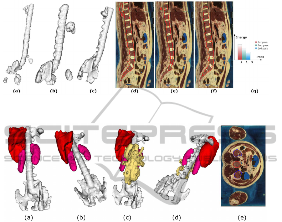
Figure 4: Multipass segmentation. Shown are the segmentation results after (a) the first pass, (b) the second pass, and (c) the
third pass. (d)-(f) Contour of the zero level set (red) after the first pass, the second pass, and the third pass, respectively. (g)
Classifier and edge field energy after each pass.
Figure 5: Segmentation in the abdomen area. (a)-(d) 3D visualization of segmented organs in the abdomen, including spine
(white), liver (red), kidney (pink), and intestine (yellow). (e) Final contours of the zero level sets in a 2D slice (red for spine,
blue for kidney).
roughly indicate which regions belong to the objects
of interest and which belong to the background. The
segmentation of liver is most challenging because
its texture is very similar to the texture of muscle
tissues. Our classifier and Gabor filter responses can
successfully distinguish them as shown in Fig. 7.
5.2 Fiber Bundle Segmentation in
Diffusion Tensor Images
Fiber bundles are coherently organized brain white
matter pathways, which can be computed from dif-
fusion tensor images. Our pipeline for fiber bundle
segmentation includes the following stages: initial
user input, classification on a 2D slice, (backward)
fiber tracking and levelset-based fiber bundle extrac-
tion, as shown in Fig. 6. At the beginning, the user
chooses a 2D image slice SL and draws a region of
interest on it. A probabilistic classifier is then trained
and used to assign probabilities to every voxel on the
slice. During backward fiber tracking, we start fiber
tracking from every voxel with fractional anisotropy
greater than 0.1. If the fiber eventually passes a voxel
p
sl
on slice SL, we propagate the probability at p
sl
to
the voxel. We adopt the adaptive fourth order Runge-
Kutta method as in (Press et al., 2002; Mori and van
Zijl, 2002) to track fiber bundles. During the final
stage, we run our levelset-based segmentation on the
entire diffusion tensor image, whose voxels have been
associated with probabilities, to finalize fiber bundle
extraction.
Fig. 6 shows an example of fiber bundle segmen-
tation. We extract corpus callosum from a volumet-
ric diffusion tensor image using our level set method.
Corpus callosum is a bridge between the left brain and
the right one. It is filled with dense fibers (Aboitiz
et al., 1992; Basser et al., 2000). The original data
is a 256×256×32 diffusion tensor image. The user
first selects a 2D image slice near corpus callosum,
VISAPP2013-InternationalConferenceonComputerVisionTheoryandApplications
392
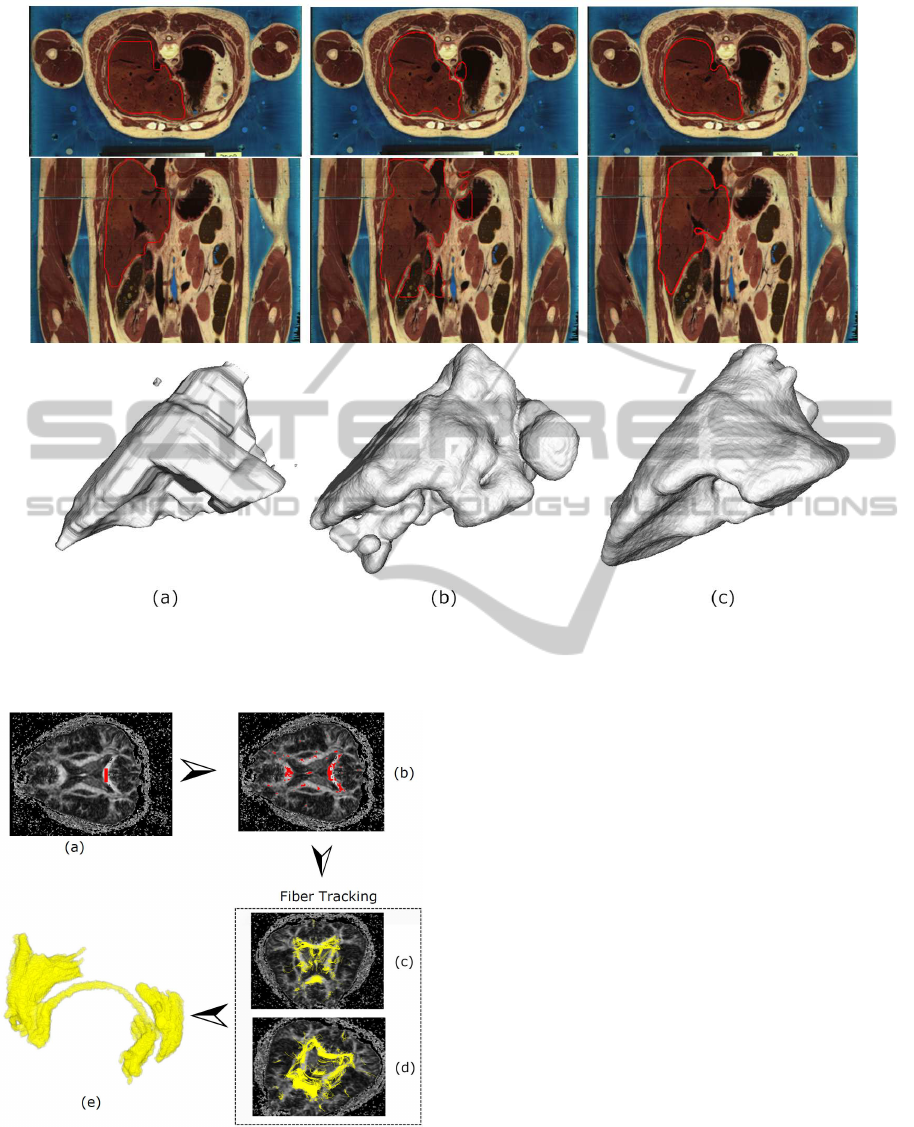
Figure 7: Segmentation Comparison. The first and second rows show segmentation results in 2D slices; the third row shows
segmentation results using 3D visualization. (a) Graphcut, (b) the algorithm from (Holtzman-Gazit et al., 2006), (c) our
method.
Figure 6: The pipeline of fiber bundle segmentation. (a)
User-drawn region on a 2D slice of a diffusion tensor im-
age, (b)initial foreground pixels chosen by the probabilistic
classifier, (c)-(d) fiber tracking, (e) fiber bundles of corpus
callosum segmented using our levelset-based method.
and draws two small rectangular regions on the slice.
The entire fiber bundle can then be extracted using our
method.
5.3 Comparisons
The level set method is a popular method in biomed-
ical image segmentation (Holtzman-Gazit et al.,
2006). We compared our segmentation algorithm
with the popular graphcut algorithm (Boykov and
Jolly, 2001) and another state-of-the-art levelset-
based algorithm in (Holtzman-Gazit et al., 2006). The
results are shown in Fig. 7. Minimization of the
graphcut energy function gives rise to faceted seg-
mentation boundaries, that do not accurately snap
to salient volume edges. Note that we also inte-
grated the same classifier with the graphcut algorithm.
Even though the graphcut segmentation result (Fig.
7(a)) significantly overlaps with our segmentation re-
sult (Fig. 7(c)), the result from our method is much
more accurate in boundarylocalization and also much
smoother.
The levelset based method in (Holtzman-Gazit
et al., 2006) is good at processing medical volume
MedicalVolumeSegmentationbasedonLevelSetsofProbabilities
393

images with thin structures. However, without the
use of discriminative classifiers and texture descrip-
tors, it could not distinguish liver tissues from muscle
tissues, as shown in Fig. 7(b).
6 CONCLUSIONS
We have presented a robust and accurate method for
biomedical image segmentation using level sets of
probabilities. Our method integrates a probabilis-
tic classifier with the level set method, making the
level set method less vulnerable to local minima. Our
method obtains a posterior probabilistic mask of an
object of interest as the segmentation result. We
further alternate classifier training and the level set
method to improve the performance of both. We have
successfully applied our method to the segmentation
of various organs and tissues in the Visible Human
dataset. Level sets of probabilities can be applied
in segmentation of three dimensional MR images as
shown in Fig. 6. Experiments and comparisons have
demonstrated the effectiveness of our method.
ACKNOWLEDGMENTS
This work was partially supported by National Natu-
ral Science Foundation of China (NSFC) (61202255).
REFERENCES
Aboitiz, F., Scheibel, A. B., Fisher, R. S., and Zaidel, E.
(1992). Fiber composition of the human corpus callo-
sum. Brain Research, 598(1-2):143–153.
Basser, P. J., Pajevic, S., Pierpaoli, C., Duda, J., and Al-
droubi, A. (2000). In vivo fiber tractography using dt-
mri data. Magnetic Resonance in Medicine, 44:354–
363.
Boykov, Y. and Jolly, M. (2001). Interactive graph cuts for
optimal boundary and region segmentation of objects
in n-d images. In Intl. Conf. Computer Vision, vol-
ume I, pages 105–112.
Cobzas, D., Birkbeck, N., Schmidt, M., and Jagersand, M.
(2007). 3d variational brain tumor segmentation using
a high dimensional feature set. In Proceedings of the
International Conference on Computer Vision, pages
1–8. IEEE.
Friedman, J., Hastie, T., and Tibshirani, R. (2000). Additive
logistic regression: a statistical view of boosting. The
Annals of Statistics, 28(2):337–407.
Hadwiger, M., Kniss, J. M., Rezk-salama, C., Weiskopf, D.,
and Engel, K. (2006). Real-time Volume Graphics. A.
K. Peters, first edition.
Holtzman-Gazit, M., Kimmel, R., Peled, N., and Goldsher,
D. (2006). Segmentation of thin structures in volu-
metric medical images. IEEE Transaction on Image
Processing, 15(2):354–363.
Liu, Y. and Yu, Y. (2012). Interactive image segmentation
based on level sets of probabilities. IEEE Transaction
on Visualization and Computer Graphics, 18(2):202–
213.
Manjunath, B. and Ma, W. (1996). Texture features for
browsing and retrieval of image data. IEEE Trans-
actions on Pattern Analysis and Machine Intelligence,
18(8):837–842.
Mori, S. and van Zijl, P. C. M. (2002). Fiber tracking: prin-
ciples and strategies - a technical review. NMR IN
BIOMEDICINE, 15:468–480.
Osher, S. J. and Fedkiw, R. P. (2003). Level Set Methods
and Dynamic Implicit Surfaces. Springer-Verlag, first
edition.
Paragios, N. and Deriche, R. (1999). Geodesic active re-
gions for supervised texture segmentation. In Pro-
ceedings of the International Conference on Computer
Vision, volume 2, pages 926–932. IEEE.
Peng, D., Merriman, B., Osher, S., Zhao, H., and Kang,
M. (1999). A pde-based fast local level set method.
Journal of Computational Physics, 155(2):410–438.
Pham, D. L., Xu, C., and Prince, J. L. (2000). Current meth-
ods in medical image segmentation. Annual Review of
Biomedical Engineering, 2:315–337.
Press, W. H., Saul A. Teukolsky, W. T. V., and Flannery,
B. P. (2002). Numerical recipes in C++: the art of sci-
entific computing. Cambridge University Press,New
York, second edition.
Schroeder, W., Martin, K., and Lorensen, B. (2004). The
Visualization Toolkit. Kitware Inc., third edition.
Sethian, J. (1999). Level Set Methods and Fast Marching
Methods. Cambridge University Press.
Tu, Z., Narr, K. L., Dollar, P., Dinov, I., Thompson, P. M.,
and Toga, A. W. (2008). Brain anatomical struc-
ture segmentation by hybrid discriminative/generative
models. IEEE Transactions on Medical Imaging,
27(4):495–508.
VISAPP2013-InternationalConferenceonComputerVisionTheoryandApplications
394
