Reinforcement Learning for Multi-purpose Schedules
Kristof Van Moffaert, Yann-Micha
¨
el De Hauwere, Peter Vrancx and Ann Now
´
e
Department of Computer Science, Vrije Universiteit Brussel, 1050 Elsene, Belgium
Keywords:
Machine Learning, Reinforcement Learning, Optimization, Multi-objective, Energy.
Abstract:
In this paper, we present a learning technique for determining schedules for general devices that focus on
a combination of two objectives. These objectives are user-convenience and gains in energy savings. The
proposed learning algorithm is based on Fitted-Q Iteration (FQI) and analyzes the usage and the users of a
particular device to decide upon the appropriate profile of start-up and shutdown times of that equipment. The
algorithm is experimentally evaluated on real-life data to discover that close-to-optimal control policies can
be learned on a short timespan of a only few iterations. Our results show that the algorithm is capable of
proposing intelligent schedules depending on which objective the user placed more or less emphasis on.
1 INTRODUCTION
Automatic control policies received a great deal of at-
tention in recent years. Combining such control poli-
cies with a low resource consumption and minimal
costs is a goal that researchers from various disci-
plines are attempting to achieve. Traditional manu-
ally designed control strategies lack predictive capa-
bilities to ensure a certain quality of service in sys-
tems that are characterized by diverse usage patterns
and user preferences. As a result, such systems do
not provide effective solutions for achieving the de-
sired resource efficiency. Moreover, such traditional
approaches typically also result in a significant risk of
temporary discomfort as part of the learning phase or
due to ill-configured systems.
In this paper we describe an approach that aims
to automatically configure product systems to user
demand patterns and their preferences. This means
tailoring the performance of devices to the specific
circumstances imposed on them by their everyday
users. By taking into account patterns in user behav-
ior and expectations, the system usage optimization
is twofold. On the one hand side, the quality of ser-
vice provided by the system to the end user, and on
the other hand the resources needed to keep the sys-
tem running. Such tailoring can be influenced by time
dependent usage patterns as well as personal or group
determined performance preferences.
Consider for instance an espresso or a coffee ma-
chine. An espresso machine has different operational
modes: on (making the beverage), idle (temporarily
heat water) and off. By default, the machine is idle.
Every couple of minutes, the machine will re-heat it’s
water supply, to always be in a state of readiness when
a user wants coffee. After office hours, the machine
should be turned off manually, to bring down power
consumption even further. Bringing the coffee ma-
chine from off to idle again in the morning mode re-
quires a warming up phase, which implies that the
machine is not immediately usable. On a typical day,
the beverage machine used in an office environment
will be turned on in the morning and remain on during
the day, being used only sporadically. During long pe-
riods of time, the machine will be idling. Consistently
turning it off after usage is a hindrance because the
machine will need to warm up each time it is switched
on again. Finding a correct control policy which op-
timizes energy consumption, without sacrificing hu-
man comfort will be the scope of the experiments de-
scribed later on.
We propose a batch Reinforcement Learning (RL)
approach that outputs a control policy based on his-
toric data of usage and user preferences. This ap-
proach avoids the overhead and discomfort typically
associated with a learning phase in reinforcement
learning while still having the benefit of being adap-
tive to changing patterns and preferences. In Section
2, we elaborate on related concepts that allow auto-
matic extracting of user patterns. Furthermore, we
present the problem setting in Section 3 and the corre-
sponding experiments in Section 4. These results are
discussed in the subsequent Section 5 and to conclude
the paper, we form conclusions obtained in Section 6.
203
Van Moffaert K., De Hauwere Y., Vrancx P. and Nowé A..
Reinforcement Learning for Multi-purpose Schedules.
DOI: 10.5220/0004187202030209
In Proceedings of the 5th International Conference on Agents and Artificial Intelligence (ICAART-2013), pages 203-209
ISBN: 978-989-8565-39-6
Copyright
c
 2013 SCITEPRESS (Science and Technology Publications, Lda.)

2 BACKGROUND AND
PRELIMINARIES
In this section, we focus on related work of techniques
concerning automatic retrieval of user patterns and
profiles.
2.1 MDPs and Reinforcement Learning
A Markov Decision Process (MDP) can be described
as follows. Let S = {s
1
, . . . , s
N
} be the state space of a
finite Markov chain {x
l
}
l≥0
and A = {a
1
, . . . , a
r
} the
action set available to the agent. Each combination of
starting state s
i
, action choice a
i
∈ A
i
and next state
s
j
has an associated transition probability T (s
j
|, s
i
, a
i
)
and immediate reward R(s
i
, a
i
). The goal is to learn
a policy π, which maps each state to an action so that
the the expected discounted reward J
π
is maximized:
J
π
≡ E
"
∞
∑
t=0
γ
t
R(s(t), π(s(t)))
#
(1)
where γ ∈ [0, 1) is the discount factor and expectations
are taken over stochastic rewards and transitions. This
goal can also be expressed using Q-values which ex-
plicitly store the expected discounted reward for every
state-action pair:
Q
∗
(s, a) = R(s, a) + γ
∑
s
0
T (s
0
|s, a)max
a
0
Q(s
0
, a
0
) (2)
So in order to find the optimal policy, one can learn
this Q-function and then use greedy action selection
over these values in every state. Watkins described
an algorithm to iteratively approximate Q
∗
. In the Q-
learning algorithm (Watkins, 1989) a large table con-
sisting of state-action pairs is stored. Each entry con-
tains the value for
ˆ
Q(s, a) which is the learner’s cur-
rent hypothesis about the actual value of Q(s, a). The
ˆ
Q-values are updated accordingly to following update
rule:
ˆ
Q(s, a) ← (1 − α
t
)
ˆ
Q(s, a) +α
t
[r + γmax
a
0
ˆ
Q(s
0
, a
0
)]
(3)
where α
t
is the learning rate at time step t and r is the
reward received for performing action a in state s.
Provided that all state-action pairs are visited in-
finitely often and a suitable evolution for the learning
rate is chosen, the estimates,
ˆ
Q, will converge to the
optimal values Q
∗
(Tsitsiklis, 1994).
2.1.1 Fitted-Q Iteration
Fitted Q-iteration (FQI) is a model-free, batch-mode
reinforcement learning algorithm that learns an ap-
proximation of the optimal Q-function (Busoniu et al.,
2010). The algorithm requires a set of input MDP
transition samples (s, a, s
0
, r), where s is the transition
start state, a is the selected action and s
0
, r are the state
and immediate reward resulting from the transition,
respectively. Given these samples, fitted Q-iteration
trains a number of successive approximations to the
optimal Q-function in an off-line fashion. The com-
plete algorithm is listed in Algorithm 1. Each itera-
tion of the algorithm consists of a single application
of the standard Q-learning update from Equation 3 for
each input sample, followed by the execution of a su-
pervised learning method in order to train the next
Q-function approximation. In the literature, the fit-
ted Q-iteration framework is most commonly used
with tree-based regression methods or with multi-
layer perceptrons, resulting in algorithms known as
Tree-based Fitted Q-iteration (Ernst et al., 2005) and
Neural Fitted-Q iteration (Riedmiller, 2005). The
FQI algorithm is particularly suited for problems with
large input spaces and large amounts of data, but
where direct experimentation with the system is diffi-
cult or costly.
Algorithm 1: Fitted Q-iteration.
ˆ
Q(s, a) ← 0 ∀s, a  Initialize approximations
repeat
T,I ←
/
0
for all samples i do  Build training set
I ← I ∪(s
i
, a
i
)  Input values
T ← T ∪ r
i
+ max
a
ˆ
Q(s
0
i
, a)  Target output value
end for
ˆ
Q ← Regress(I,T)  Train supervised learning
method
until Termination
return
ˆ
Q  Return final Q-values
3 PROBLEM SETTING
In our experiments, we recorded the presences of the
employees in a small firm together with the usage of a
particular small-office device, in this case an espresso
maker. As in most companies, there is nobody partic-
ularly designated for turning unnecessary equipment
off at unnecessary moments in time and as every-
body is eager to have their beverage ready when they
please, the general policy of the espresso maker con-
sists of a 24/7 operational time.
3.1 Presence and Usage Probabilities
In the experiments we conducted below, we extracted
the presence and usage of six individual users of the
coffee maker. The presence probabilities for each of
the six users are collected using software tools that
ICAART2013-InternationalConferenceonAgentsandArtificialIntelligence
204

analyze network activity in the firm. As most em-
ployee actually turn their computer off during ab-
sence, this technique was adequate to monitor the
presences without requiring direct, manual interaction
of the employees with an specific authentication sys-
tem, such as a system with badge recognition. The
probability distribution, extracted from this data was
collected for a period of one month and is depicted
in Figure 1. From these distributions, we notice that
users 2 and 3 regularly leave their computer on for
the entire day. This behavior introduces noise into
the system, but should not cause too much additional
problems for this technique to come up with an ap-
propriate schedule for the espresso maker. At around
11h to 12h, most people tend to leave for lunch and
thus less activity is spotted on the network. In the af-
ternoon, at around 17h, on average occasions, most of
the employees tend to leave their office and shut down
their computer. Occasionally, some employees seem
to be working late.
The other type of information needed is the usage
of the particular device. The usage of the espresso
maker is measured by the number of cups being drank
at the office. Similar to the manner presence was be-
ing monitored, we opted for a measuring technique
that did not require manual input from the user. To
obtain usage information, we relied on an appliance
monitoring device
1
that records the power consump-
tion of the coffee maker every six seconds. By analyz-
ing this data, the timestamps at which a user actually
requested coffee could be retrieved. It is important to
notice that no information is collected on who is ac-
tually requesting coffee, i.e. only the time-dependent
information is recorded. This data is collected for the
same period of time as the presence information and is
presented in Figure 2. Given the fact that the espresso
maker can only be operated when employees are ac-
tually present at the office, there is a peak in morning,
from 8h to 10h, when most of the beverages is being
consumed. In this period of time, around 1.3 to 1.4
cups of coffee are being requested, which is in fact
quite minimal. While in the afternoon, the usage is
diminished with a small peak at 14h and starting from
18h, there were no recordings of people consuming
any beverages.
For each of the six users, a series of working
days are generated using the presence distributions as
a probability distribution together with noise added
from a Normal distribution, while for the usage dis-
tribution a Poisson (Haight, 1967) distribution is em-
ployed to generate different usages for different days.
The Poisson distribution is especially tailored for ex-
1
We conducted our experiments with the EnviR appli-
ance monitor
pressing the probability of a given number of events
occurring in a fixed interval of time or space if these
events occur with a known average rate and indepen-
dently of the time since the last event. The combina-
tion of the two graphs allow us to generate a variety
days with simulated presences and usages up to the
level of 10 minutes, i.e. for each simulated day 144
individual data points are generated.
0 2 4 6 8 10 12 14 16 18 20 22
0
0.2
0.4
0.6
0.8
1
Hour
Probability
User 1
User 2
User 3
User 4
User 5
User 6
Figure 1: The probability distribution for each of the six
individual users on their presence.
0 2 4 6 8 10 12 14 16 18 20 22
0
0.2
0.4
0.6
0.8
1
1.2
1.4
Hour
Usage
Usage
Figure 2: The distribution of the company’s drinking behav-
ior based on historical data.
3.2 A General Device Model
Another important part of our experimental setting is
the model used to represent the device, being con-
trolled. This model should be both general and spe-
cific enough to capture all aspects of any household
device. A Markov Decision Process, as introduced
in Section 2.1, is specifically tailored for representing
the behavior of a particular household device. In total,
two possible actions and three states are presented in
an MDP that would cover most, if not all household
equipment. The three states or modes of the MDP
are ’on’, ’off ’ or ’booting’, where the latter represents
the time needed before the actual operational mode is
reached. The action space A of our MDP is limited
to two distinct, deterministic actions, i.e. the agent
can either decide to press a switch or relay that alters
the mode of the machine or it can decide do leave the
mode of the machine unchanged and do nothing. The
former action is a simplification to two separate ac-
tions ’turn on’ and ’turn off ’.
An aspect of the MDP that we did not cover yet
ReinforcementLearningforMulti-purposeSchedules
205

is the immediate reward R
a
(s, s
0
) received after tran-
sitioning to state s
0
from state s by action a. These
rewards are a combination of two objectives, i.e.. an
energy consumption penalty and a reward given by
the user. The latter is a predefined constant for dif-
ferent situations that can occur. For instance, when
the machine is turned off but at the same time a user
wanted coffee, then, the current policy does not meet
that specific user’s profile and the policy is manually
overruled. Although, for a general audience this is
not necessary a bad policy when the algorithm has de-
ducted that in fact the probability of somebody want-
ing a beverage was very low and from an energy-
consumption point of view, it was not interesting to
have the device turned on. In such a case, the system
is provided with a negative feedback signal indicating
the user’s inconvenience. On the other hand, when
the device is turned on at the same time that a user
requested a beverage, then the policy actually suits
the current user and the system anticipated well on
the expected usage. In those cases, positive reward is
provided to the system.
The former reward signal is a measure indicating
quality of a certain action a in terms of power con-
sumption. These rewards are device-dependent and
allow the learning algorithm on top to learn over time
whether leaving the device in idle mode is energy re-
ducing enough for the current state s of S or if a shut-
down is needed. By specifying a certain cost for cold-
starting the device, in according to the real-life cost,
the algorithm could also learn to power the device
on x minutes before a timeslot where a lot of con-
sumption is expected. In general, the learning algo-
rithm will have to deduct which future timeslots are
expected to have a positive difference between the
consumption reward signal and the user satisfaction
feedback signal. For the moment, these two reward
signals are combined by scalarization.
To conclude, our MDP is graphically repre-
sented in Figure 3 and is mathematically for-
malized as follows: M= < S, A, P, R >, where
S = {On, Off, Booting} and A = {Do nothing,
press switch}. The transitions between the differ-
ent states are deterministic, resulting in a probability
function P that is shown in Figure 3. The reward func-
tion R is device-specific and we will elaborate this
function in the sections below.
4 EXPERIMENTS
At each of data points, representing a point in time,
the FQI algorithm, described in Section 2.1.1, will de-
cide which action to take from the action space given
On Off
Booting
Press switch
Press switch
Boot for x minutes
Do nothing
Do nothing
Figure 3: A general model for almost every household de-
vice.
the current hour, interval of 10 minutes and presence
set, with 24, 6 and 2
6
possible values, respectively.
These figures results in a large state space of 9,216
possible combinations. In our setting, the FQI algo-
rithm was first trained with data of one single sim-
ulated day and the control policy was tested for one
new day after every training step, whereafter this test
sample was also added to the list of training samples
to increase the training set’s size. Thus, an on-line
learning setting was created. In our experiments, we
opted for the Tree-Based FQI algorithm with a classi-
fication and regression tree or CARTand we averaged
our results over 10 individual trials.
For the reward signals in our MDP M, we mim-
icked the properties of a real-life espresso maker into
our simulation framework. Using the same appliance
monitoring equipment, we have tried to capture the
real-life power consumption of the device under dif-
ferent circumstances. After measuring the power con-
sumption of the machine for a few weeks, we came to
the following conclusions:
• We noticed that, for our industrial coffee maker,
the start-up time was very fast. In just over one
minute, the device heated the water up to the boil-
ing temperature and the beverage could be served.
The power consumption of actually making coffee
is around 940 Watts per minute.
• When the machine was running in idle mode, the
device is only using around 2 Watts most of the
time. However, every ten minutes, the coffee
maker re-heated its water automatically. On av-
erage, this results in an energy consumption of 5
Watts per minute in idle mode.
• The device does not consume any power when
turned off.
The reward signals to identify the user’s satisfaction
or inconvenience, when the device was turned on and
off, respectively, can be tuned to obtain schedules for
ICAART2013-InternationalConferenceonAgentsandArtificialIntelligence
206

the coffee maker that focus on either or both.
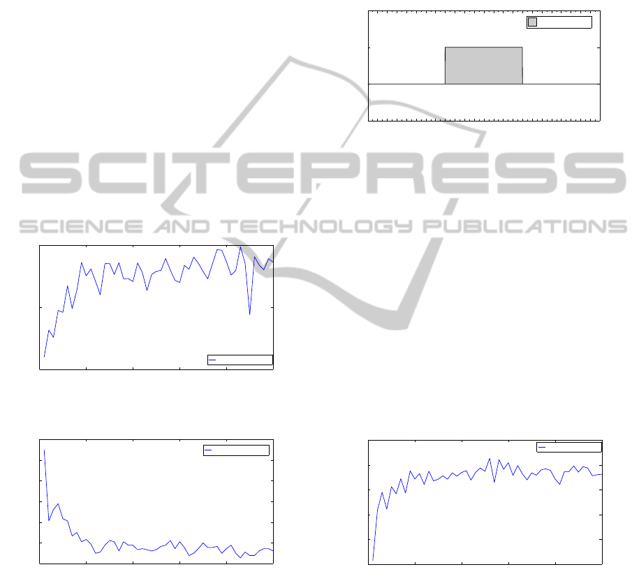
4.1 A User-oriented Schedule
In a first experiment, we defined a large positive and
negative value for the user satisfaction reward (+0.5)
and the user inconvenience cost (−0.4), respectively.
With these rewards in place, we ran the FQI algorithm
for 50 simulation days. Although the learning curve
in Figure 4 is still fluctuating significantly at the final
learning days, we see that the good performance is
being reached from day 20. This observation is con-
firmed in Figure 5, where we plotted the number of
manual overrides that occurred on each day. Initially,
the number of manual overrides per day is around
10, where in final iterations, around 2 overrides are
needed. In the initial learning phases, the algorithm
tries out a series of different start-up and shutdown
times for the coffee maker. Upon observing the state
of the machine and the feedback from the users, it
tries to refine its schedule by improving and adjusting
the schedule to their needs.
0 10 20 30 40 50
−5
0
5
Day
Reward
Collected reward
Figure 4: The learning curve for learning a schedule that
focusses on satisfying the convenience of the users.
0 10 20 30 40 50
0
2
4
6
8
10
12
Day
Overrides
Manual overrides
Figure 5: The number of human interventions needed that
involve a manual start-up of the coffee maker diminishes as
learning proceeds.
Currently a setting is created that focuses heavily
on the keeping an accepted level of user-friendliness
compared to energy-efficiency, the system proposes
the schedule of Figure 6. Although some people tend
to be present before 8h, the algorithm decides to have
the coffee maker turned on at 8h to be prepared for
the high peak in usage (Figure 2). Although not that
many beverages are being consumed in the afternoon,
a lot of employees are still present at the office, which
increases the chance of somebody using the machine.
This makes the suggested schedule result in a very
user-friendly schedule taking the gains of keeping an
accepted level of user-friendliness over the potential
economical benefits of turning the device off for a
small period of time.
0 2 4 6 8 10 12 14 16 18 20 22
Off
On
Hour
State
Device’s state
Figure 6: The user-friendly policy decides to have the coffee
maker turned on at 8h and turned off at 16h.
4.2 An Energy-oriented Schedule
Instead of focusing on the users of the actual system,
one could prefer to find a policy that focusses more
on keeping the energy consumption down. A radical
schedule that takes into consideration only the power
consumption side of the story could be have the de-
vice turned off all the time and let the users them-
selves have the task of starting-up the system accord-
ing to their needs. However, such a schedule would be
of little to no value in any real-life situation. There-
fore, we conduct the same experiment as in Section
4.1, but decrease the user’s influence on the learned
policy. The new rewards are 0.35 and −0.35 to define
user convenience and inconvenience, respectively.
0 10 20 30 40 50
−6
−4
−2
0
2
4
Day
Rewad
Collected reward
Figure 7: The learning curve for an energy-oriented sched-
ule.
After around the same number of training days as
in the previous experiment, a stable performance is
obtained (Figure 7). The number of manual overrides
(Figure 8) stays acceptably low because the final pol-
icy in Figure 9 focuses on leaving the device turned on
at the most critical time of the day, i.e. the morning
when at the same time most people tend to be present
and most of the beverages are being consumed.
ReinforcementLearningforMulti-purposeSchedules
207

0 10 20 30 40 50
0
2
4
6
8
10
12
Day
Overrides
Manual overrides
Figure 8: The number of manual overrides decrease as
learning proceeds. Although this metric is currently not be-
ing focussed on too much, the number of manual overrides
stays low.
0 2 4 6 8 10 12 14 16 18 20 22
Off
On
Hour
State
Device state
Figure 9: The final policy obtained turns the device on from
8h to 10h50, while leaving it off during the less occupied
afternoon.
4.3 Energy Consumption
The three schedules, i.e. the original always-on, the
user-oriented and the energy-oriented policy, can also
be compared in terms of economical gains. Given
the actual cost of 0.22 eper Kilowatt hour (kWh) and
an average consumption of the espresso machine in
stand-by mode of around 300 Watts per hour, the re-
sults are listed in Table 1. From these figures, we
deduct an annual saving of around 66.6% and 88.2%
for the user-oriented and energy-oriented profiles, re-
spectively, compared to the initial setting of always
leaving the device on.
5 DISCUSSION AND RELATED
WORK
In the first experiment we showed how the FQI al-
gorithm quite easily managed to generalize from the
large state-space. The schedule proposed in that par-
ticular setting might seem trivial, but applying such a
schedule would already be a significant money saver
in most offices. On the other hand, the second ex-
periment, where we placed less emphasis on the ob-
jective indicating the convenience of the user, the ob-
tained schedule is much more interesting. Although
most people tend to be present from 8h to 17h, it has
analyzed the combination of the presence and the us-
age information on the long run to conclude that the
timespan from 8h to little before 11h is the most crit-
ical one. As the most critical timeslot of the general
working day is covered, also the number of manual
overrides remains acceptably low, i.e. only two man-
ual interventions are needed during the entire day.
Thus, when the device is being used at later times that
day, the user is still free to manual overrule the sched-
ule, but the algorithm will not suggest such an action
itself.
The economical savings one can accomplish by
implementing these schedules are compared to the
company’s initial schedule which was to leave the de-
vice always on as nobody took responsibility, are of
course significant. A potential cost saving of 385.7 e
and 510.3 e for the user-oriented and energy-oriented
profile, respectively, could be obtained if an automatic
control device applied one of these proposed sched-
ules. Besides the economical cost, there is also the
wear and tear of device itself that should be taken into
consideration. It is obvious that an always-on profile
is not beneficial for the lifetime and durability of the
device and neither is a profile that rapidly switches
between operational modes.
Previous research has applied the Fitted-Q algo-
rithm mainly in single-objective optimal control prob-
lems (e.g. (Busoniu et al., 2010; Riedmiller, 2005;
Ernst et al., 2005)). More recently, (Castelletti et al.,
2012) also introduced a multi-objective FQI version,
which is capable of approximating the Pareto frontier
in learning problems with multiple objectives, and ap-
plied this algorithm to learn operation policies for wa-
ter reservoir management. None of these works, how-
ever, consider the problem of user interactions and
taking into account end-user preferences. To the best
of our knowledge this paper presents the first appli-
cation of FQI in a setting which includes both a cost
function and direct user feedback.
Several authors have considered other reinforce-
ment learning algorithms in problem settings related
to those presented in this paper. In (Dalamagkidis
et al., 2007), an on-line temporal difference RL con-
troller is developed to control a building heating sys-
tem. The controller uses a reinforcement signal which
is the weighted combination of 3 objectives: energy
consumption, user comfort and air quality. On-line
RL algorithms have also been applied to the problem
of energy conservation in wireless sensor networks,
often in combination with other objectives such as
satisfying certain routing criteria (see e.g. (Liu and
Elhanany, 2006; Mihaylov et al., 2010)). Finally,
(Khalili et al., 2009) apply Q-learning to learn user
preferences in a smart home application setting. Their
ICAART2013-InternationalConferenceonAgentsandArtificialIntelligence
208

Table 1: The economical properties of the three schedules.
Always-on User-oriented Energy-oriented
Operational hours per day 24h 8h 2h50
Cost per month (e) 48.22 16.08 5.68
Cost per year (e) 578.56 192.86 68.25
system is able to adapt to (time-varying) user prefer-
ences regarding ambient light and music settings, but
does not take into other criteria such as account en-
ergy consumption.
6 CONCLUSIONS
In this paper, we have presented our results on ap-
plying Reinforcement Learning (RL) techniques on
real-life data to come-up with appropriate start-up and
shutdown decisions for multi-criteria environments.
These two criteria are user convenience and energy.
We have seen that the FQI algorithm integrates very
well into such a multi-objective environment and by
specifying emphasis on each of the different objec-
tives, one can obtain schedules for everyone’s needs.
The aspect of this work that requires the most oppor-
tunities for future research is the manner how both
reward signals can be combined in a more intelligent
way by multi-objective techniques. As in many of to-
day’s attempts in the RL research landscape, combin-
ing multiple reward signals is limited to scalarization
techniques and no aspects of Pareto dominance rela-
tionships are incorporated. Our next step is to incor-
porate RL with multi-objective techniques and apply
these techniques in a similar real-life environment we
have presented here.
To conclude, we have shown how one can fairly
easily come up with an application of RL using histor-
ical data and cheap monitoring devices. In the near fu-
ture, one of our intentions is to shift these simulations
out of the virtual world and to design a real-world sys-
tem using automated control devices that apply these
schedules in the same office where the measurements
took place.
ACKNOWLEDGEMENTS
This research is supported by IWT-SBO project PER-
PETUAL. (grant nr. 110041).
REFERENCES
Busoniu, L., Babuska, R., De Schutter, B., and Ernst, D.
(2010). Reinforcement Learning and Dynamic Pro-
gramming using Function Approximators, volume 39
of Automation and Control Engineering Series. CRC
Press.
Castelletti, A., Pianosi, F., and Restelli, M. (2012). Tree-
based fitted q-iteration for multi-objective markov de-
cision problems. In Proceedings International Joint
Conference on Neural Networks (IJCNN 2012).
Dalamagkidis, K., Kolokotsa, D., Kalaitzakis, K., and
Stavrakakis, G. (2007). Reinforcement learning for
energy conservation and comfort in buildings. Build-
ing and Environment, 42(7):2686 – 2698.
Ernst, D., Geurts, P., and Wehenkel, L. (2005). Tree-based
batch mode reinforcement learning. Journal of Ma-
chine Learning Research, 6:503–556.
Haight, F. (1967). Handbook of the Poisson distribution.
Publications in operations research. Wiley.
Khalili, A., Wu, C., and Aghajan, H. (2009). Autonomous
learning of users preference of music and light ser-
vices in smart home applications. In Proceedings
Behavior Monitoring and Interpretation Workshop at
German AI Conf.
Liu, Z. and Elhanany, I. (2006). A reinforcement learning
based mac protocol for wireless sensor networks. Int.
J. Sen. Netw., 1(3/4):117–124.
Mihaylov, M., Tuyls, K., and Now
´
e, A. (2010). Decen-
tralized learning in wireless sensor networks. Lecture
Notes in Computer Science, 4865:60–73.
Riedmiller, M. (2005). Neural fitted q iteration – first ex-
periences with a data efficient neural reinforcement
learning method. In In 16th European Conference on
Machine Learning, pages 317–328. Springer.
Tsitsiklis, J. (1994). Asynchronous stochastic approxima-
tion and q-learning. Journal of Machine Learning,
16(3):185–202.
Watkins, C. (1989). Learning from Delayed Rewards. PhD
thesis, University of Cambridge.
ReinforcementLearningforMulti-purposeSchedules
209