2D-PAGE Texture Classification using Support Vector Machines
and Genetic Algorithms
An Hybrid Approach for Texture Image Analysis
Carlos Fernandez-Lozano
1
, Jose A. Seoane
1
, Pablo Mesejo
2
, Youssef S. G. Nashed
2
,
Stefano Cagnoni
2
and Julian Dorado
1
1
Information and Communications Technologies Department, University of A Coruña, Coruña, Spain
2
Department of Information Engineering, University of Parma, Province of Parma, Parma, Italy
Keywords: Texture Analysis, Feature Selection, Electrophoresis, Support Vector Machines, Genetic Algorithm.
Abstract: In this paper, a novel texture classification method from two-dimensional electrophoresis gel images is
presented. Such a method makes use of textural features that are reduced to a more compact and efficient
subset of characteristics by means of a Genetic Algorithm-based feature selection technique. Then, the
selected features are used as inputs for a classifier, in this case a Support Vector Machine. The accuracy of
the proposed method is around 94%, and has shown to yield statistically better performances than the
classification based on the entire feature set. We found that the most decisive and representative features for
the textural classification of proteins are those related to the second order co-occurrence matrix. This
classification step can be very useful in order to discard over-segmented areas after a protein segmentation
or identification process.
1 INTRODUCTION
Proteomics is the study of protein properties in a
cell, tissue or serum aimed at obtaining a global
integrated view of disease, physiological and
biochemical processes of cells and regulatory
networks. One of the most powerful techniques,
widely used to analyze complex protein mixtures
extracted from cells, tissues, or other biological
samples, is two-dimensional polyacrylamide gel
electrophoresis (2D-PAGE). In this method, proteins
are classified by molecular weight (MWt) and iso-
electric point (pI) using a controlled laboratory
process and digital imaging equipment.
Since the beginning of proteomic research, 2D-
PAGE has been the main protein separation
technique, even before proteomics became a reality
itself. The main advantages of this approach are its
robustness, its parallelism and its unique ability to
analyse complete proteins at high resolution,
keeping them intact and being able to isolate them
entirely (Rabilloud, Chevallet et al. 2010). However,
this method has also several drawbacks as its very
low effectiveness in the analysis of hydrophobic
proteins, as well as its high sensitivity to dynamic
range (i.e. quantitative ratio between the rarest
protein expressed in a sample and the most abundant
one) and quantitative distribution issues (Lu, Vogel
et al. 2007). The outcome of the process is an image
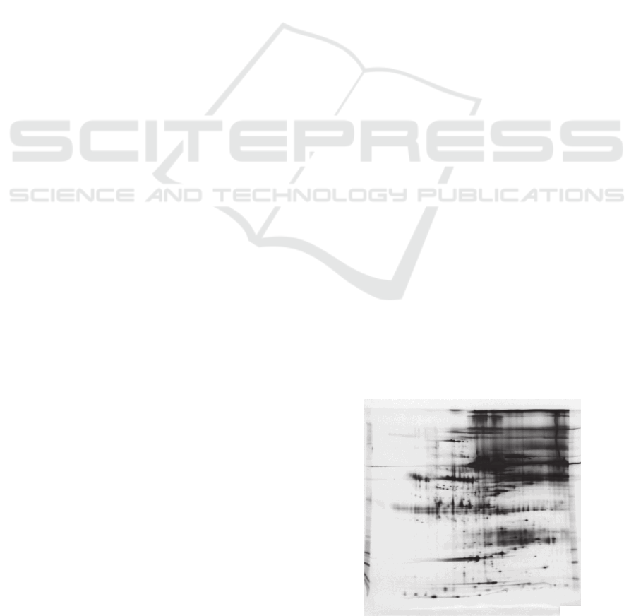
like the one showed in Figure 1.
Figure 1: Example image used to detect potential serum
protein biomarkers in children with fetal alcohol
syndrome. 512x512 pixels. 8 bit. 340 microns/pixel.
Taken from Lemkin public use dataset.
Dealing with this kind of images is a difficult
5
Fernandez-Lozano C., Seoane J., Mesejo P., S. G. Nashed Y., Cagnoni S. and Dorado J..
2D-PAGE Texture Classification using Support Vector Machines and Genetic Algorithms - An Hybrid Approach for Texture Image Analysis.
DOI: 10.5220/0004187400050014
In Proceedings of the International Conference on Bioinformatics Models, Methods and Algorithms (BIOINFORMATICS-2013), pages 5-14
ISBN: 978-989-8565-35-8
Copyright
c
2013 SCITEPRESS (Science and Technology Publications, Lda.)

task because there is not a commonly accepted
ground truth (Lemkin ; Marten). Another aspect that
makes the work difficult from a computer vision
point of view, is that both protein images and
background noise seem to follow a Gaussian
distribution (Tsakanikas and Manolakos 2009). The
inter- and intra-operator variability in manual
analysis of these images is also a big drawback
(Millioni et al., 2010).
The aim of this paper is to demonstrate that there
is enough texture information in 2D-electrophoresis
images to discriminate proteins from noise or
background. In this work the most representative
group of textural features are selected using Genetic
Algorithms.
2 THEORETICAL
BACKGROUND AND RELATED
WORK
The method proposed in this work intends to assist
in 2D-PAGE image analysis by studying the textural
information present within them. To do so, a novel
combination of Genetic Algorithms (Holland, 1975)
and Support Vector Machines (Vapnik, 1979) is
presented. In this section, the main techniques used
are briefly introduced and explained.
One of the most important characteristics used
for identifying objects or regions of interest in an
image is texture, related with the spatial (statistical)
distribution of the grey levels within an image
(Haralick et al., 1973). Texture is a surface’s
property and can be regarded as the almost regular
spatial organization of complex patterns, always
present even if they could exist as a non-dominant
feature. Other approaches (i.e. Structural which
represents texture by well-defined primitives and a
hierarchy of spatial arrangements. Model based
which using fractal and stochastic models, attempt to
interpret and image texture. Transform method such
as Fourier, Gabor or Wavelet transforms), within a
texture analysis, have been applied and a good
review can be found in (Materka and Strzelecki,
1998); (Tuceryan and Jain, 1999).
Genetic Algorithms (GAs) are search techniques
inspired by Darwinian Evolution and developed by
Holland in the 1970s (Holland, 1975). In a GA, an
initial population of individuals, i.e. possible
solutions defined within the domain of a fitness
function to be optimized, is evolved by means of
genetic operators: selection, crossover and mutation.
The selection operator ensures the survival of the
fittest, while the crossover represents the mating
between individuals, and the mutation operator
introduces random modifications. GAs possesses
effective exploration and exploitation capabilities to
explore the search space in parallel, exploiting the
information about the quality of the individuals
evaluated so far (Goldberg, 1989). Using the
crossover operator, GA combines the features of
parents to produce new and better solutions, which
preserve the parents’ best characteristics. By making
use of the mutation operator, new information is
introduced in the population in order to explore new
and promising areas of the search space. Another
strategy known as elitism, which is a variant of the
general process of constructing a new population, is
to allow better organisms from the current
generation to carry over the next, remaining
untalterd. At the end of the process, it is expected
that the population of solutions converges to the
global optimum.
Vapnik introduces Support Vector Machines
(SVMs) in the late 1970s on the foundation of
statistical learning theory (Vapnik, 1979). The basic
implementation deals with two-class problems in
which data are separated by a hyperplane defined by
a number of support vectors. This hyperplane
separates the positive from the negative examples, to
orient it such that the distance between the boundary
and the nearest data point in each class is maximal;
the nearest data points are used to define the
margins, known as support vectors (Burges, 1998).
These classifiers have also proven to be
exceptionally efficient in classification problems of
higher dimensionality (Chapelle et al., 1999);
(Moulin et al., 2004), because of their ability to
generalize in high-dimensional spaces, such as the
ones spanned by texture patterns. SVM uses
different non-linear kernel functions, like
polynomial, sigmoid and radial basis function,
where the nonlinear SVM maps the training samples
from the input spaces into a higher-dimensional
feature space via a mapping function (Burges, 1998).
With respect to related work, the authors were
not able to find any other work in the literature
handling with evolutionary computation in
combination with texture analysis in 2D-
electrophoresis images; however, one article
describes a discriminant partial least squares
regression (PLSR) method for spot filtering in 2D-
electrophoresis (Rye and Alsberg, 2008). They use a
set of parameters to build a model based on texture,
shape and intensity measurements using image
segments from gel segmentation. As regards texture
information, they have focused on descriptors
BIOINFORMATICS2013-InternationalConferenceonBioinformaticsModels,MethodsandAlgorithms
6

related to the noisy surface texture of unwanted
artefacts and concluded that their textural features
allow them to distinguish noisy features from protein
spots. In this work, five out of the eleven second-
order textural features, from the Grey Level Co-
Ocurrence Matrix (GLCM) firstly proposed by
Haralick, are used, and five new textural features
accounting for intensity relationships among sets of
three pixels. They distinguish proteins in the image
by using shape information, since cracks and
artefacts in gel surface deviate from a circular shape.
Besides that, a degree of Gaussian fit is calculated as
an indication of whether the image segment
corresponds to a protein or an artefact. Thereby
textural features are used for noise and crack
detection and as a complement for spot
segmentation. Finally, the 17 initial variables are
reduced to five PLSR components to account for
85% of the total variation with respect to the
response factor, and 82% of the total variation in the
data matrix.
3 MATERIALS
In order to generate the dataset, ten 2D-PAGE
images enough representative of different types of
tissues and different experimental conditions were
used. These images are similar to the ones used by
G.-Z. Yang (Imperial College of Science,
Technology and Medicine, London). It is important
to notice that Hunt et al. (Hunt et al., 2005)
determined that 7-8 is the minimum acceptable
number of samples for a proteomic study.
For each image, 50 regions of interest (ROIs)
representing proteins and 50 representing no-
proteins (noise, black non-protein regions, and
background) were selected to build a training set
with 1000 samples in a double-blind process in the
way that two clinicians select as many ROIs as they
considered and after that, within the common ROIs
clinicians selected proteins which are representatives
(isolated, overlapped, big, small, darker, etc.). For
each element, as will be seen later, 296 texture
features are computed.
The ROIs were selected taking into consideration
that, for each manually selected protein, there is an
area of influence surrounding it. It means that, once
the clinician has selected a protein, the ROI is
slightly bigger than the visible dark surface of such a
protein. This assumption is made because texture
could exist not only in the darkest grey levels but
also in the grey levels closest to white.
As said before, proteins seem to fit a Gaussian
peak, and ideally the center of the protein is in the
darkest zone of that peak. This approach prevents
the loss of information caused by neglecting the
lowest values of the inverted protein (grey levels
closest to white) that also fit the Gaussian peak. This
information could be useful to classify a protein or
to discard it.
4 PROPOSED METHOD
This paper goes further than related work in the
texture analysis of 2D-electrophoresis images,
studying the ability of textural features to
discriminate not only cracks from proteins but
background and no-protein dark spots as well.
The first step in texture analysis is texture feature
extraction from the ROIs. With a specialized
software called Mazda (Szczypinski et al., 2007),
296 texture features are computed for each element
in the training set. Various approaches have
demonstrated the effectiveness of this software
extracting textural features in different types of
medical images (Bonilha et al., 2003); (Létal et al.,
2003); (Mayerhoefer et al., 2005); (Harrison et al.,
2008); (Szymanski et al., 2012).
These features (Szczypiski et al., 2009), reported
in Table 1, are based on:
Image histogram
Co-ocurrence matrix: information about the grey
level value distribution of pairs of pixels with a
preset angle and distance between each other.
Run-length matrix: information about sequences
of pixels with the same grey level values in a
given direction.
Image gradients: spatial variation of grey level
values.
Autoregressive models: description of texture
based on statistical correlation between
neighbouring pixels.
Wavelet analysis: information about the image
frequency content at different scales.
Thus, from each ROI, texture information was
analyzed by extracting first and second-order
statistics, spatial frequencies, co-occurrence matrices
and two other statistical methods as autoregressive
model and wavelet based analysis, preserving the
original gray-level and spatial resolution on all runs.
Histogram-related measures conform the first-order
statistics proposed by Haralick (Haralick et al.,
1973) but second-order statistics are those derived
from the Spatial Distribution Grey-Level Matrices
2D-PAGETextureClassificationusingSupportVectorMachinesandGeneticAlgorithms-AnHybridApproachfor
TextureImageAnalysis
7

(SDGM). First-order statistics depend only on
individual pixel values and can be computed from
the histogram of pixel intensities in the image.
Second-order statistics depend on pairs of grey
values and on their spatial resolution. Additionally a
group of features derived from the textural ones is
also calculated, but cannot be used for texture
characterization such as the area of the ROI.
Table 1: Textural features extracted and used in this work.
Group Features
Histogram
Mean, variance, skewness, kurtosis,
percentiles 1%, 10%, 50%, 90% and
99%
Absolute
Gradient
Mean, variance, skewness, kurtosis and
percentage of pixels with nonzero
gradient
Run-length
Matrix
Run-length nonuniformity, grey-level
nonuniformity, long-run emphasis,
short-run emphasis and fraction of
image in runs
Co-ocurrence
Matrix
Angular second moment, contrast,
correlation, sum of squares, inverse
difference moment, sum average, sum
variance, sum entropy, entropy,
difference variance and difference
entropy
Autoregressive
Model
Theta: model parameter vector, four
parameters; Sigma: standard deviation
of the driving noise
Wavelet
Energy of wavelet coefficients in
subbands at successive scales; max
four scales, each with four parameters
All these feature sets were included in the
dataset. The normalization method applied was the
one set by default in Mazda: image intensities were
normalized in the range from 1 to Ng=2
k
, where k is
the number of bits per pixel used to encode the
image under analysis.
Two solutions are available for decreasing
dimensionality: extraction of new features derived
from the existing ones and selection of relevant
features to build robust models. In order to extract a
feature set from the problem data, principal
component analysis (PCA) has been commonly
used. In this work, GA is aimed at finding the
smallest feature subset able to yield a fitness value
above a threshold. Besides optimizing the
complexity of the classifier, feature selection may
also improve the classifiers’ quality. In fact,
classification accuracy could even improve if noisy
or dependent features are removed.
GAs for feature selection were first proposed by
Siedlecki and Skalansky (Siedlecki and Sklansky,
1989). Many studies have been done on GA for
feature selection since then (Kudo and Sklansky,
1998), concluding that GA is suitable for finding
optimal solutions to large problems with more than
40 features to select from.
GA for feature selection could be used in
combination with a classifier such SVM, k-nearest
neighbor (KNN) or artificial neural network (ANN),
optimizing it. In terms of classification accuracy
with imaging problems, SVMs have shown good
performance with textural features (Kim et al.,
2002); (Li et al., 2003); (Buciu et al., 2006), but also
KNN (Jain 1997) and hybrid approaches, which use
a combination of both classifiers (Zhang et al.,
2006), have obtained good results. Other techniques
use GA to optimize both the feature selection and
classifier parameters (Huang and Wang, 2006);
(Manimala et al., 2011).
In our method, based on both GA and SVM,
there are not a fixed number of variables. As the GA
continuously reduces the number of variables that
characterize the samples, a pruned search is
implemented. Each individual in the genetic
population is described by p genes (using binary
encoding). The fitness function (1) considers not
only the classification results but also the number of
variables used for such a classification, so it is
defined as the sum of two factors, one related to the
classification results and another to the number of
variables selected. In (1) the number of genes with a
true binary value (feature selected) is represented by
numberActiveFeatures. Regarding classification
results, it apparently gives better results taking into
account the F-measure than only using the accuracy
obtained with image features (Müller et al., 2008);
(Tamboli and Shah, 2011). F-measure (2) is a
function made up of the recall (true positives rate or
sensitivity: proportion of actual positives which are
correctly identified as such) and precision (or
positive predictive value: proportion of positive test
results that are true positives) measurements.
1
(1)
2.
.
(2)
Therefore individuals with less active genes are
favored. Once the reduced feature dataset is
generated, a parametric test is made to evaluate the
adequacy of the feature selection process.
5 EXPERIMENTAL RESULTS
The test set is composed of ten representative
BIOINFORMATICS2013-InternationalConferenceonBioinformaticsModels,MethodsandAlgorithms
8

images for the different types of proteomic available
images, and for each one of them, 50 protein and 50
non-protein ROIs have been extracted to generate a
dataset with 1000 elements, that was divided
randomly in 800 elements, of which 600 elements
are used for training and 200 elements are used for
validation (inside the GA feature selection process)
and finally, 200 elements for test. Once the GA
finishes, the best individual found (the one with
lowest fitness value) is tested, using a 10-fold cross
validation (10-fold CV), to calculate the error of the
proposed model using the full and reduced datasets.
Then, a test set is used in order to evaluate the
adequacy of the reduction process.
Parameters domains of the feature selection
method are set as given in Table 2. These parameters
were initially adjusted based on the literature.
Table 2: Domain of GA tested parameters and operators.
Item Domain
Population Size From 100 to 250
Elitism From 0 to 2 %
Crossover probability From 80 to 98 %
Mutation probability From 1 to 5 %
Crossover operators
One-point crossover, two-point
crossover, scattered, arithmetic,
heuristic
Selection function
Uniform, roulette and
tournament
Mutation function Uniform, Gaussian
Different experiments have been performed and
the final combination set the population size to 250
individuals, with no elite, a 95% crossover
probability, a 2% mutation probability, with
crossover scattered, tournament selection and
mutation uniform.
SVM parameters domains are set as given in
Table 3. The best results are shown in Table 4 in the
Appendix section. In the last column of this Table,
the final reduced textural features selected by the
GA-SVM combination is presented for each
configuration.
To evaluate the performance of this method,
there are several number of well-known accuracy
measures for a two-class classifier in the literature
such as: classification rate (accuracy), precision,
sensitivity, specificity, F-score, Area Under an ROC
Curve (AUC), Youden’s index, Cohen’s kappa,
likelihoods, discriminant power, etc. An
experimental comparison of performance measures
for classification could be found in (Ferri et al.,
2009). In (Huang and Ling, 2005), the authors
proposed that AUC is a better measure in general
than accuracy when comparing classifiers and in
general. The most common measures used for their
simplicity and successful application are the
classification rate and Cohen’s kappa measures.
Table 5 shows the results for classification rate
(accuracy), AUC, F-measure, Youden’s and
unweighted Cohen’s Kappa for each kernel. For this
problem, all the measures consider the same ranking,
and the best kernel function is the linear one. For
each kernel, Table 5 in the Appendix section shows
each feature in their textural membership group.
Table 3: SVM parameters domain.
Item Domain
Kernel function
Linear, quadratic,
polynomial and
Gaussian radial basis.
Gaussian radial basis sigma From 0.1 to 10
Gaussian radial basis C From 1 to 100
Polynomial order From 3 to 10
Method to find the hyperplane Quadratic programming
Among others, Mazda computes the area for
each ROI. This feature merely indicates the number
of pixels used for parameters computation. Being
strictly with a texture analysis process, it cannot be
used for texture characterization. With linear,
polynomial (order 3), and RBF (C=100 and
sigma=10) kernels, no textural features are selected
in order to select the most representative ones for
solving the classification problem. The presented
results seem to indicate that the textural group with
more representatives in 2D-PAGE images is the Co-
ocurrence matrix Group (second-order statistics).
As the proposed work intends to evaluate the
textural information present in a 2D-PAGE image,
the RBF(2) kernel function is selected as the most
accurate for solving this problem, since this kernel
has only textural features and the best rate in the
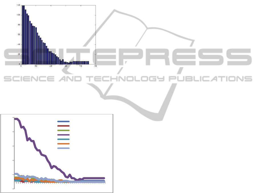
accuracy evaluation. After 45 generations, the GA
stopped because the stall condition was reached as
the best individual fitness value had not improved in
10 consecutive generations. Figure 2 reports the
number of features selected in each generation.
Figure 3 shows the evolution of the total number of
features, grouped by membership and selected
during GA generation.
We evaluate the reduced textural feature dataset
with the 200 elements reserved from the original
training set with the RBF (2) kernel, by calculating
the areas under the receiver operating characteristic
curves (AUC-ROCs) and a 10-fold CV for
separating the elements, using the Libsvm classifier
implementation (Chang and Lin, 2011) in Weka
(Hall et al., 2009) and comparing the results with the
2D-PAGETextureClassificationusingSupportVectorMachinesandGeneticAlgorithms-AnHybridApproachfor
TextureImageAnalysis
9
same classifier using the full dataset. Thus, we have
obtained samples composed by 10 AUC-ROC
measures. AUC-ROC area can be seen as the
capacity to be sensitive and specific at the same
time, in the sense that the bigger is the AUC-ROC,
the more accurate is the model. The ROC curve is a
graphical plot of the sensitivity against 1-specificity
as the detector threshold, or a parameter which
modifies the balance between sensitivity and
specificity.
Figure 2: Number of variables used in each GA
generation.
We use the RBF kernel with different gamma
values to check if there is a significant improvement
when the reduced dataset is used.
Figure 3: Evolution of feature number by group
membership during generations.
In order to use a parametric test, it is necessary to
check the independence, normality and
heteroscedasdicity (Sheskin, 2011). In statistics, two
events are independent when the fact that one occurs
does not modify the probability of the other one. An
observation is normal when its behaviour follows a
normal or Gaussian distribution with a certain value
of mean and variance. The heteroscedasticity
indicates the existence of a violation of the
hypothesis of equality of variances (García et al.,
2009).
With respect to the independence condition, we
separate the data using 10-fold CV. We perform a
normality analysis using the Shapiro-Wilk test
(Shapiro and Wilk, 1965) with a level of confidence
alpha=0.05, for the Null Hypothesis that the data
come from a normally distributed population. Null
hypothesis was rejected. The observed data fulfill
the normality condition, a Bartlett test (Bartlett,
1937) is performed in order to evaluate the
heteroscedasticity with a level of confidence
alpha=0.05.
A corrected paired Student’s t-test could be
performed in Weka (Hall et al., 2009), with a level
of confidence alpha=0.05, for the Null Hypothesis
that there are no differences between the average
values obtained by both methods. Results in average,
with standard deviation in brackets for AUC-ROC
are 0.94 (0.07) for the reduced dataset, and 0.55
(0.34) for the full dataset and the corrected paired
Student’s t-test determines that there is a significant
improvement in using the reduced dataset. The
reduced dataset has better accuracy result than the
full dataset. Even more, the corrected paired
Student’s t-test evaluates this improvement as
significant with an alpha=0.05.
Finally, the reduced textural features are the
following:
Perc. (1)%
S(2,-2)DifEntrp
S(5,0) Correlat and InvDfMom
S(0,5) DifVarnc
S(5,5) SumEntrp
The 1% histogram percentile is a first order textural
feature calculated from the original image, taking
into account the intensity value and the frequency of
every pixel. Difference entropy, correlation, inverse
difference moment, difference variance and sum
entropy are second-order textural features. These
features evaluate the co-occurrence relationship
between pixels of the original image at a given
distance and angle. Hence, there is a relationship in
the co-occurrence matrix that allows the
discrimination of a protein in 2D-PAGE images.
6 SUMMARY AND
CONCLUSIONS
To the best of our knowledge, this is the first work
in which the classification of proteins texture in two-
dimensional electrophoresis gel images is tackled
using Evolutionary Computation, Support Vector
‐10
10
30
50
70
90
1 4 7 101316192225283134374043
Histogram(9)
Absolutegradient(5)
Run‐lengthmatrix(20)
Coocurrencematrix(221)
Autoregressivemodel(5)
Wavelet(15)
Notexturalfeatures(22)
BIOINFORMATICS2013-InternationalConferenceonBioinformaticsModels,MethodsandAlgorithms
10

Machines and Textural Analysis. In fact, this paper
demonstrates the existence of enough textural
information to discriminate proteins from noise and
background, as well as to show the potential of
SVMs in proteomic classification problems.
A new dataset with six features, starting from the
296 original ones, is created without loss of
accuracy, and the most representative textural group
is the Co-ocurrence matrix Group (second-order
statistics). In our experiments, the GLCM has
appeared as the best approximation for a good
classification of proteins in two-dimensional gel
electrophoresis. According to SVM, the 1%
histogram percentile, difference entropy, correlation,
inverse difference moment, difference variance and
sum entropy, are the most representative features for
solving this problem. A proper statistical test has
determined that there is a significant improvement in
using this reduced feature set with respect to the full
feature set.
ACKNOWLEDGEMENTS
This work is supported by the General Directorate of
Culture, Education and University Management of
the Xunta de Galicia (Ref. 10SIN105004PR). Pablo
Mesejo and Youssef S.G. Nashed are funded by the
European Comission (MIBISOC Marie Curie Initial
Training Network, FP7 PEOPLE-ITN-2008, GA n.
238819).
REFERENCES
Bartlett, M. S. (1937). "Properties of Sufficiency and
Statistical Tests." Proceedings of the Royal Society of
London. Series A, Mathematical and Physical
Sciences 160(901): 268-282.
Bonilha, L., E. Kobayashi, et al. (2003). "Texture Analysis
of Hippocampal Sclerosis." Epilepsia 44(12): 1546-
1550.
Buciu, I., C. Kotropoulos, et al. (2006). "Demonstrating
the stability of support vector machines for
classification." Signal Processing 86(9): 2364-2380.
Burges, C. J. C. (1998). "A tutorial on support vector
machines for pattern recognition." Data Mining and
Knowledge Discovery 2(2): 121-167.
Chang, C. C. and C. J. Lin (2011). "LIBSVM: A Library
for support vector machines." ACM Transactions on
Intelligent Systems and Technology 2(3).
Chapelle, O., P. Haffner, et al. (1999). "Support vector
machines for histogram-based image classification."
IEEE Transactions on Neural Networks 10(5): 1055-
1064.
Ferri, C., J. Hernádez-Orallo, et al. (2009). "An
experimental comparison of performance measures for
classification." Pattern Recognition Letters 30(1): 27-
38.
García, S., A. Fernández, et al. (2009). "A study of
statistical techniques and performance measures for
genetics-based machine learning: Accuracy and
interpretability." Soft Computing 13(10): 959-977.
Goldberg, D. (1989). Genetic Algorithms in Search,
Optimization, and Machine Learning, Addison-
Wesley Professional.
Hall, M., E. Frank, et al. (2009). "The WEKA data mining
software: an update." SIGKDD Explor. Newsl. 11(1):
10-18.
Haralick, R. M., K. Shanmugam, et al. (1973). "Textural
features for image classification." IEEE Transactions
on Systems, Man and Cybernetics smc 3(6): 610-621.
Harrison, L., P. Dastidar, et al. (2008). "Texture analysis
on MRI images of non-Hodgkin lymphoma."
Computers in Biology and Medicine 38(4): 519-524.
Holland, J. H. (1975). Adaptation in natural and artificial
systems: an introductory analysis with applications to
biology, control, and artificial intelligence, University
of Michigan Press.
Huang, C. L. and C. J. Wang (2006). "A GA-based feature
selection and parameters optimizationfor support
vector machines." Expert Systems with Applications
31(2): 231-240.
Huang, J. and C. X. Ling (2005). "Using AUC and
accuracy in evaluating learning algorithms." IEEE
Transactions on Knowledge and Data Engineering
17(3): 299-310.
Hunt, S. M. N., M. R. Thomas, et al. (2005). "Optimal
Replication and the Importance of Experimental
Design for Gel-Based Quantitative Proteomics."
Journal of Proteome Research 4(3): 809-819.
Jain, A. (1997). "Feature selection: evaluation, application,
and small sample performance." IEEE Transactions on
Pattern Analysis and Machine Intelligence
19(2): 153-
158.
Kim, K. I., K. Jung, et al. (2002). "Support vector
machines for texture classification." IEEE
Transactions on Pattern Analysis and Machine
Intelligence 24(11): 1542-1550.
Kudo, M. and J. Sklansky (1998). "A comparative
evaluation of medium- and large-scale feature
selectors for pattern classifiers." Kybernetika 34(4):
429-434.
Lemkin, P. F. ”The LECB 2D page gel image data set”,
from http://www.ccrnp.ncifcrf.gov/users/lemkin.
Létal, J., D. Jirák, et al. (2003). "MRI 'texture' analysis of
MR images of apples during ripening and storage."
LWT - Food Science and Technology 36(7): 719-727.
Li, S., J. T. Kwok, et al. (2003). "Texture classification
using the support vector machines." Pattern
Recognition 36(12): 2883-2893.
Manimala, K., K. Selvi, et al. (2011). "Hybrid soft
computing techniques for feature selection and
parameter optimization in power quality data mining."
Applied Soft Computing Journal 11(8): 5485-5497.
2D-PAGETextureClassificationusingSupportVectorMachinesandGeneticAlgorithms-AnHybridApproachfor
TextureImageAnalysis
11

Marten, R. "Marten Lab Proteomics Page." 2012, from
http://www.umbc.edu/proteome/image_analysis.html
Materka, A. and M. Strzelecki (1998). "Texture analysis
methods-A review." Technical University of Lodz,
Institute of Electronics. COST B11 report.
Mayerhoefer, M. E., M. J. Breitenseher, et al. (2005).
"Texture analysis for tissue discrimination on T1-
weighted MR images of the knee joint in a multicenter
study: Transferability of texture features and
comparison of feature selection methods and
classifiers." Journal of Magnetic Resonance Imaging
22(5): 674-680.
Millioni, R., S. Sbrignadello, et al. (2010). "The inter- and
intra-operator variability in manual spot segmentation
and its effect on spot quantitation in two-dimensional
electrophoresis analysis." Electrophoresis 31(10):
1739-1742.
Moulin, L. S., A. P. Alves Da Silva, et al. (2004).
"Support vector machines for transient stability
analysis of large-scale power systems." IEEE
Transactions on Power Systems 19(2): 818-825.
Müller, M., B. Demuth, et al. (2008). An evolutionary
approach for learning motion class patterns. 5096
LNCS: 365-374.
Rabilloud, T., M. Chevallet, et al. (2010). "Two-
dimensional gel electrophoresis in proteomics: Past,
present and future." Journal of Proteomics 73(11):
2064-2077.
Rye, M. B. and B. K. Alsberg (2008). "A multivariate spot
filtering model for two-dimensional gel
electrophoresis." Electrophoresis 29(6): 1369-1381.
Shapiro, S. S. and M. B. Wilk (1965). "An analysis of
variance test for normality (complete samples)."
Biometrika 52(3-4): 591-611.
Sheskin, D. J. (2011). Handbook of Parametric and
Nonparametric Statistical Procedures, Taylor and
Francis.
Siedlecki, W. and J. Sklansky (1989). "A note on genetic
algorithms for large-scale feature selection." Pattern
Recognition Letters 10(5): 335-347.
Szczypinski, P. M., M. Strzelecki, et al. (2007). MaZda - A
software for texture analysis.
Szczypiski, P. M., M. Strzelecki, et al. (2009). "MaZda-A
software package for image texture analysis."
Computer Methods and Programs in Biomedicine
94(1): 66-76.
Szymanski, J. J., J. T. Jamison, et al. (2012). "Texture
analysis of poly-adenylated mRNA staining following
global brain ischemia and reperfusion." Computer
Methods and Programs in Biomedicine 105(1): 81-94.
Tamboli, A. S. and M. A. Shah (2011). A Generic
Structure of Object Classification Using Genetic
Programming. Communication Systems and Network
Technologies (CSNT), 2011 International Conference
on.
Tsakanikas, P. and E. S. Manolakos (2009). "Improving 2-
DE gel image denoising using contourlets."
Proteomics 9(15): 3877-3888.
Tuceryan, M. and A. Jain (1999). Texture analysis.
Handbook of pattern recognition and computer vision,
World Scientific Publishing Company, Incorporated. 2.
Vapnik, V. N. (1979). Estimation of dependences based on
empirical data [in Russian]. Nauka, English
translation Springer Verlang, 1982.
Zhang, H., A. C. Berg, et al. (2006). SVM-KNN:
Discriminative nearest neighbor classification for
visual category recognition.
BIOINFORMATICS2013-InternationalConferenceonBioinformaticsModels,MethodsandAlgorithms
12
APPENDIX
Table 4: Results with different SVM kernel types.
TP FN FFP TN Acc AUC F-Meas Y’s Kapp Nvar Texture features
RBF(1) 90 10 18 82 0.86 0.86 0.8653 0.72 0.72 8
S(2,0)InvDfMom
S(0,3)SumAverg
S(0,3)DifVarnc
S(4,-4)Contrast
S(0,5)SumEntrp
S(0,5)DifEntrp
S(5,5)SumEntrp
S(5,-5)Entropy
RBF(2) 94 6 17 83
0.88
5
0.88 0.8909 0.77 0.77 6
Perc.01%
S(2,-2)DifEntrp
S(5,0)Correlat
S(5,0)InvDfMom
S(0,5)DifVarnc
S(5,5)SumEntrp
Linear 95 5 11 89 0.92 0.92 0.9268 0.85 0.85 6
Skewness
S(2,2)Correlat
S(4,0)InvDfMom
_Area_S(0,4)
S(5,0)Contrast
_Area_S(5,-5)
Poli(3) 87 13 19 81 0.84 0.84 0.844 0.68 0.68 16
Kurtosis
S(1,-1)Contrast
S(1,-1)DifEntrp
S(0,2)DifEntrp
S(0,4)SumAverg
S(4,-4)Correlat
S(4,-4)SumVarnc
S(5,0)InvDfMom
S(0,5)SumOfSqs
S(0,5)InvDfMom
S(0,5)SumEntrp
45dgr_GLevNoU
_AreaGr
GrKurtosis
WavEnLH_s-2
WavEnLH_s-4
RBF(100;10) 94 6 18 82 0.88 0.88 0.8867 0.76 0.76 8
_Area_S(0,1)
S(2,0)InvDfMom
_Area_S(5,0)
S(5,0)InvDfMom
S(0,5)InvDfMom
S(5,-5)DifEntrp
Horzl_GLevNonU
WavEnLH_s-4
2D-PAGETextureClassificationusingSupportVectorMachinesandGeneticAlgorithms-AnHybridApproachfor
TextureImageAnalysis
13

Table 5: Study of texture parameters between best SVM kernels in accuracy.
Histogram
Absolute gradient
Run-length matrix
Co-occurence matrix
Autoregresivve model
Wavelet
No texture feature
RBF(1)
S(2,0)InvDfMom
S(0,3)SumAverg
S(0,3)DifVarnc
S(4,-4)Contrast
S(0,5)SumEntrp
S(0,5)DifEntrp
S(5,5)SumEntrp
S(5,-5)Entropy
RBF(2) Perc.01%
S(2,-2)DifEntrp
S(5,0)Correlat
S(5,0)InvDfMom
S(0,5)DifVarnc
S(5,5)SumEntrp
Linear Skewness
S(2,2)Correlat
S(4,0)InvDfMom
S(5,0)Contrast
_Area_S(0,4)
_Area_S(5,-5)
Poli(3) Kurtosis GrKurtosis 45dgr_GLevNonU
S(1,-1)Contrast
S(1,-1)DifEntrp
S(0,2)DifEntrp
S(0,4)SumAverg
S(4,-4)Correlat
S(4,-4)SumVarnc
S(5,0)InvDfMom
S(0,5)SumOfSqs
S(0,5)InvDfMom
S(0,5)SumEntrp
WavEnLH_s-2
WavEnLH_s-4
_AreaGr
RBF(100;10)
Horzl_GLevNonU
S(2,0)InvDfMom
S(5,0)InvDfMom
S(0,5)InvDfMom
S(5,-5)DifEntrp
WavEnLH_s-4
_Area_S(0,1)
_Area_S(5,0)
BIOINFORMATICS2013-InternationalConferenceonBioinformaticsModels,MethodsandAlgorithms
14
