Facial Landmarks Localization Estimation by Cascaded Boosted

Regression

Louis Chevallier

, Jean-Ronan Vigouroux

, Alix Goguey

1,2

and Alexey Ozerov

Technicolor, Cesson-S

evign

e, France

Ensimag, Saint-Martin d’H

eres, France

Keywords:

Face Landmarks Localization, Boosted Regression.

Abstract:

Accurate detection of facial landmarks is very important for many applications like face recognition or analy-

sis. In this paper we describe an efﬁcient detector of facial landmarks based on a cascade of boosted regressors

of arbitrary number of levels. We deﬁne as many regressors as landmarks and we train them separately. We

describe how the training is conducted for the series of regressors by supplying training samples centered on

the predictions of the previous levels. We employ gradient boosted regression and evaluate three different

kinds of weak elementary regressors, each one based on Haar features: non parametric regressors, simple lin-

ear regressors and gradient boosted trees. We discuss trade-offs between the number of levels and the number

of weak regressors for optimal detection speed. Experiments performed on three datasets suggest that our

approach is competitive compared to state-of-the art systems regarding precision, speed as well as stability of

the prediction on video streams.

1 INTRODUCTION

Facial landmarks detection is an important step in

face analysis. Indeed, performance of face recogni-

tion or characterization systems (Everingham et al.,

2006) greatly depends on the accuracy of this mod-

ule. Accordingly, much work has been devoted to the

problem of accurate and robust localization of facial

landmarks. The importance of the required accuracy

level depends on the ﬁnal application. For example,

for applications requiring a ﬁne analysis of faces like

lips-reading, a very precise localization of landmarks

is needed. Typically, such high precision performance

is required on near frontal faces; non-frontal positions

are less likely to be subjected to these analyzes. More-

over, when this analysis involves motion video, tem-

poral stability at a given precision rate is useful.

Most of state of the art landmark detectors (Cootes

et al., 2001; U

r et al., 2012; Cao et al., 2012;

Dantone et al., 2012; Vukadinovic and Pantic, 2005)

are formulated as optimization or regression prob-

lems in some high-dimensional space (e.g., dozens

of thousands of features). Thus, the precision of

these approaches is limited by feature resolution. Us-

ing higher feature resolution (i.e., a feature space

of much higher dimension), will in general not lead

to improved precision due to limited training data,

but instead entail over-ﬁtting problems. We pro-

pose a new approach that allows increased feature

resolution while keeping the feature space dimen-

sion unchanged, leading to higher landmark detec-

tion accuracy. This is achieved by using a cascade

of boosted regressors, where the features used at each

cascade level are extracted from a restricted area sur-

rounding the corresponding landmark estimated by

the previous levels of the cascade. We also discuss

trade-offs between the number of cascades and the

number of weak regressors for an optimal detection

speed/precision ratio.

Our main contributions are:

1. A fast and accurate landmark position estimation

algorithm, based on boosted weak regressors and

Haar features extracted from the surrounding area,

and a cascaded estimation scheme iterating on

narrowing areas around each landmark.

2. A comprehensive assessment of the proposed

estimator with regards to standard benchmarks,

databases and state of the art landmark estima-

tors, including an evaluation of its spatial stabil-

ity. This is a new feature to our knowledge which

is of great importance for the applications we are

considering.

3. The ﬂexibility of the proposed approach allows

adjustment of the accuracy vs. computational load

513

Chevallier L., Vigouroux J., Goguey A. and Ozerov A..

Facial Landmarks Localization Estimation by Cascaded Boosted Regression.

DOI: 10.5220/0004192705130519

In Proceedings of the International Conference on Computer Vision Theory and Applications (VISAPP-2013), pages 513-519

ISBN: 978-989-8565-47-1

 2013 SCITEPRESS (Science and Technology Publications, Lda.)

by simply varying the number of cascades.

The paper is organized as follows: related work and

the proposed approach are described respectively in

sections 2 and 3. Sections 4 and 5 are devoted to eval-

uation of performance and temporal stability. Some

conclusions are drawn in section 6.

2 RELATED WORK

The problem of predicting the location of facial

landmarks consists in estimating the vector S =

, y

, ...x

, y

, x

, y

]

comprising N pairs of 2D co-

ordinates based on the appearance of the face. To

minimize ||S −

S||

, where

S denotes an estimate,

most of the existing approaches use optimization

techniques (Cristinacce and Cootes, 2008; U

et al., 2012) where the prediction is obtained as a

solution of some optimization criterion, or regres-

sion techniques (Dantone et al., 2012; Valstar et al.,

2010) where a function directly produces the predic-

tion. Our approach follows the second direction.

Regarding data modeling, most approaches rely

on both shape modeling representing a priori knowl-

edge about landmarks locations and texture model-

ing corresponding to values of pixels surrounding the

landmarks in the image itself, i.e., the posterior obser-

vations.

Active Shape Models (ASM) (Cootes et al., 1995)

is a popular hybrid approach that uses a statistical

model describing the shape (set of landmarks) of

faces together with models of the appearance (tex-

ture) of landmarks. The prediction is iteratively up-

dated to ﬁt an example of the object in a new image.

The shapes are constrained by the Point Distribution

Model (PDM) (Kass et al., 1988) to vary only in ways

seen in a training set of labeled examples. Active Ap-

pearance Models (AAM) (Cootes et al., 2001) are an

extension of the ASM approach. In AAM, a global

appearance model is used to optimize the shape pa-

rameters. Among the weaknesses frequently pointed

out for this approach are the need for images of suf-

ﬁciently high resolution, and the sensitivity to initial-

ization. Our regression approach using Haar features

computed over the face area, can, on the contrary,

work with small images–in theory as small as the grid

used for deﬁning the set of Haar features–in our case

17x17, yielding 13920 features. Moreover, as a re-

gression approach there is no iterative search process

to be initialized.

A straightforward approach to landmark detec-

tion is based on using independently trained detectors

for each facial landmark. For instance the AdaBoost

based detectors and its modiﬁcations have been fre-

quently used (Viola and Jones, 2001). If applied in-

dependently, the individual detectors often fail to pro-

vide a robust estimate of the landmark positions be-

cause of the weakness of local evidence. This can be

solved by using a prior on the geometrical conﬁgura-

tion of landmarks.

Valstar et al. (Valstar et al., 2010) proposed trans-

forming the detection problem into a regression prob-

lem. They deﬁne a regression algorithm, based on

Support Vector Regression, BoRMan, to estimate the

positions of the feature points from Haar features

computed at locations with maximum a priori prob-

abilities. A Belief Propagation algorithm is used to

improve the estimation of the target points, using a

Markov Random Field modeling the relative positions

of the points. Series of estimations are performed, by

adding Gaussian noise to the current target estimation,

and retaining the median of the predictions as the ﬁnal

estimation.

In (Everingham et al., 2006), a facial landmark de-

tector is described which is based on the independent

training of a local appearance model and the deforma-

tion cost of the Deformable Part Model–a structure

which captures spatial relation between landmarks.

The former relies on an AdaBoost classiﬁer using

Haar like features. The latter consists of a genera-

tive model using a mixture of Gaussian trees. In our

evaluation section, we use an implementation of this

system, which represents an optimization based solu-

tion to landmark detection.

Another approach based on regression for deter-

mining landmarks localization is described in (Cao

et al., 2012). In this work, explicit multiple regression

is used to directly predict landmarks localization. All

landmarks coordinates (the shape) are predicted si-

multaneously by the regressor. The design relies on a

cascaded structure: a top level boosted regressor uses

weak regressors that are themselves boosted. These

primary regressors use weak fern regressors: regres-

sion trees with a ﬁxed number of leaves. In contrast

with this system, our system consists of as many re-

gressors as landmarks to be predicted. While (Cao

et al., 2012) described a hierarchical structure, the

structure of our system is a true cascade of regressors

similar to the classiﬁers cascade proposed by (Viola

and Jones, 2001) in their face detector.

3 LANDMARK POSITION

ESTIMATION BY CASCADED

BOOSTED REGRESSION

We propose to estimate the position of the landmarks

VISAPP2013-InternationalConferenceonComputerVisionTheoryandApplications

514

by using boosting and cascading techniques that lead

to a fast and accurate result. The prediction of the

coordinates (x, y) of each landmark is done using a

boosted regressor, based on Haar features computed

on the detected face. A more precise localization is

obtained using cascaded predictors. Each landmark

is predicted independently of the others, instead of

using a shape-based approach, as in (Lanitis et al.,

1997; Cootes et al., 2001; Cristinacce and Cootes,

2008; U

r et al., 2012), and for each landmark

the x and y coordinates are predicted independently.

Actually, even if each landmark is predicted indepen-

dently, a shape constraint is implicitly taken into ac-

count by the ﬁrst regressor since the features used by

this regressor are extracted from the totality of the

face area. A ﬁnal test could be made to detect and

correct grossly erroneous landmarks. We believe that

this approach is robust to partial occlusion, since vari-

ability of one landmark does not perturb the position

of the others.

In contrast to (Valstar et al., 2010) we do not

regress from different starting points, and take the me-

dian position as an estimator. We build a series of es-

timations of the positions of the landmarks, designed

to converge to the sought landmark with high preci-

sion. At each step the regressor operates on increas-

ingly narrow windows.

The image measurements used in our system are

Haar features. This choice has the advantage that inte-

gral representations of images were readily available

since they are typically required by the ubiquitous Vi-

ola and Jones face detector (Viola and Jones, 2001)

we are using. The Haar features are deﬁned based on

a regular grid mapped on the shrinking image area to

be analyzed. We set the size of the grid to 17 × 17

cells and we use eight Haar feature shapes (see ﬁg-

ure 1). Scaling and translating them results in a total

of 13,920 Haar features.

Figure 1: The eight Haar features used

3.1 The First Level Regressor

The ﬁrst level regressor is a boosted regressor, using

the algorithms described in (Friedman, 2001).

For the clarity of presentation we consider the case

where we have only one coordinate of one landmark

to predict for each image. Let G be a set of N im-

ages, and y

be the coordinate of the landmark on im-

age i; the coordinates are measured in pixels from

the top-left corner of the detection box. We have at

our disposal a set of measurements (Haar features)

on each image, used by the weak regressors and we

want to create the most efﬁcient strong predictor of

the landmark coordinate, from a linear combination

of weak predictors. Here the weak predictors consist

of least-square ﬁtted linear predictors using Haar fea-

tures computed on the detected face (Viola and Jones,

2001).

The strong predictor is built iteratively as follows.

Let F be a matrix such that F

i j

is the value of the

feature F

on image i. Let Y

(n)

be a vector con-

taining the values to be predicted at iteration n. At

ﬁrst step Y

(1)

is initialized to the coordinates to pre-

dict: Y

(1)

= Y , i.e., the vector of all the y

. We

predict Y

(n)

from F

using a standard linear predic-

tor:

(n)

= a

+ b

. The prediction error is E

(n)

−

(n)

= Y

(n)

− a

− b

, and the mean error is

(n)

k. The feature minimizing this error,

is selected as n

weak predictor. The predictions

are subtracted from the value to predict, with a given

weight w

set between 0.1 and 1, and the new value

to predict is thus:

(n+1)

= Y

(n)

− w

− b

This is iterated p times and results in a Linear strong

predictor of the form:

(p)

(i) =

∑

k=1



+ b



3.2 Next Regression Levels

The estimation of the position of a landmark can be

improved by using the ﬁrst estimation to re-center a

window around the landmark of interest. This is the

basis of our cascading process (see ﬁgure 2.)

The prediction window on the ﬁrst level is the

window detected by the face detector. In the second

and subsequent levels it is a smaller window centered

on the landmark position predicted by the previous

level. For the size of the successive windows we use

a decreasing ratio applied to the original face bound-

ing box : 1.0, 0.8, 0.6, 0.4 for the four ﬁrst levels.

The levels of the cascade are therefore trained se-

quentially. The predictions of the previous level are

used to train the next level.

FacialLandmarksLocalizationEstimationbyCascadedBoostedRegression

515

Figure 2: Three successive steps of regression for the Left

Mouth Corner.

3.3 Other Weak Regressors

As an alternative to Linear predictors for weak regres-

sors we consider Non-Parametric weak-regressors. In

this case, we bin the values of each feature F

and we

estimate y

by the mean of Y for the images falling

in the same bin as F

i j

. The boosting algorithm is ap-

plied as previously on the residual. This is somewhat

equivalent to ferns (Doll

ar et al., 2010) using only one

feature.

We have also experimented with gradient boosted

trees (GBT) as weak regressors. Those regressors

combining many Haar features were expected to pro-

vide more expressive power. Given the number of

training image samples – ca. 5,000 – compared to

the number of features (13,920), the challenge was to

prevent over-ﬁtting. Optimal parameters were found

through cross validation and we set the number of

trees and maximal depth so that the total number of

leaves (Haar features) were the same as in the two

previous methods. In this experiment we are using 30

Haar features per weak regressor. The training time

per landmark with 4 cascades is 8 minutes on an octo-

core 3GHz Intel processor.

We compare the merit of these three boosted weak

regressors by testing them on the BioID database (Je-

sorsky et al., 2001) using four cascades (see table 1.)

Table 1: Percentage of tested images below error threshold

on BioID dataset with three different weak regressors pre-

dicting the right of mouth corner.

Percent. of tested images 25% 50% 75%

GBT 2.2% 3.4% 5.0%

Linear 2.7% 4.2% 6.5%

Non Parametric 3.0% 4.8% 8.4%

We notice that GBT clearly outperforms the two

other approaches.

3.4 Parameters Settings

Our approach uses two important parameters for

training: the number of weak regressors and the num-

ber of cascade levels. In order to ﬁnd the optimal

choice we have tested several trade-offs presented in

table 2.

Table 2: Error threshold at 50% of tested images on BioID

dataset with respect to weak regressors number and cascade

levels.

# levels

# weaks

15 30 45 60

1 0.057 0.044 0.041 0.038

2 0.047 0.039 0.036 0.034

3 0.042 0.037 0.034 0.032

4 0.040 0.037 0.033 0.032

Of course the greater the computation effort,

the lower the error, but for a given computation

load (i.e., the total number of Haar features which

is proportional to the product numberO f Weaks ×

numberO f Levels), say 90, we can see that two lev-

els and 45 weak regressors is the best choice.

4 EVALUATION OF

PERFORMANCE

4.1 Evaluation Methodology

The models trained as described in the previous sec-

tion were applied on three publicly available data sets

with a manually labeled ground truth:

1. BioID (Jesorsky et al., 2001) is a very popular

dataset containing 1,521 frontal face images with

moderate variations in light condition and pose.

2. The PUT (Kasi

nski et al., 2008) dataset has 9,971

faces. The main source of face appearance vari-

ations comes from changes in poses and expres-

sions .

3. The MUCT (Milborrow et al., 2010) dataset has

3,755 faces. It provides some diversity of lighting,

age and ethnicity.

The set of landmarks provided by these databases

are all different, so we retained a set of nine land-

marks found on all three datasets and for which there

is a good agreement regarding actual landmark posi-

tions: right and left corners of mouth, inner and outer

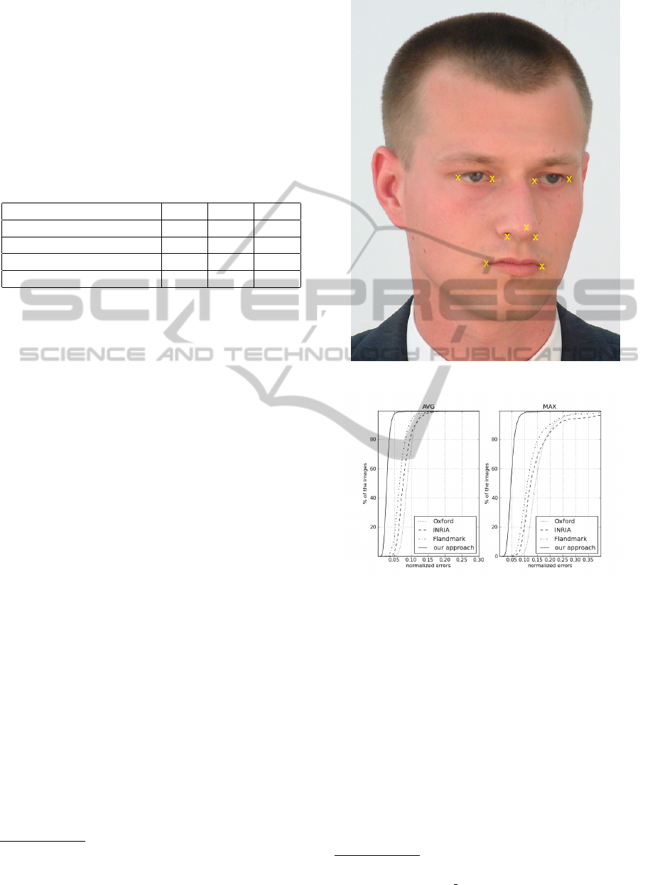
corners of eyes, nose and nostrils (see ﬁgure 3.)

Our evaluation methodology consists of training

our system with half of the images of each dataset

and testing it on the rest. We use an evaluation met-

rics proposed in (Cootes et al., 2001) and deﬁned as

follows:

∑

i=1

where d

is the Euclidean distance between the ground

truth landmark and the predicted one and s is the inter-

ocular distance. n = 9 is the number of landmarks.

VISAPP2013-InternationalConferenceonComputerVisionTheoryandApplications

516

4.2 Results

The systems against which we benchmarked our sys-

tem are FLandmark (U

r et al., 2012), Oxford (Ev-

eringham et al., 2006), CLM (Cristinacce and Cootes,

2008), Kumar (Belhumeur et al., 2011), Valstar (Val-

star et al., 2010) and Cao (Cao et al., 2012). The IN-

RIA system is a variant of (Everingham et al., 2006)

trained with a different training dataset.

Table 3: Percentage of tested images below the average er-

ror threshold on BioID dataset.

Percent. of tested images 25% 50% 75%

FLandmark 5.4% 5.5% 7.0%

Our system 2% 2.6% 3.2%

CLM 2.5% 4.5% 6.5%

Valstar 1.5% 3% 5%

We compare our system with recent systems for

which the implementation was available

. For some

others, we use the ﬁgures reported in corresponding

papers on the same datasets: In the curves on ﬁgures 4

and 5 the error curve corresponds to the average error

and to the maximum error observed on all the land-

marks.

The obtained precision on PUT and MUCT im-

ages (ﬁgure 5) are not as good as on BioID (ﬁgure 4)

because the pose of faces varies much more.

5 EVALUATION OF TEMPORAL

STABILITY

5.1 Motivation

In practice, the accuracy of landmark prediction is

limited by the modeling restriction, noise in the an-

notation and inherent ambiguity of the localization of

facial landmark. 3% seems to be a performance that

will be difﬁcult to outperform.

If a perfect accuracy cannot be reached, for some

applications, it is important that the detector be as sta-

ble as possible. For example, the output of a landmark

detector might be used as input of a speaking/non-

speaking classiﬁer, which decides whether or not a

visible face is currently speaking. Thus, if the land-

marks are used to analyze the face (evolution of the

mouth height or width), the noise due to the predictor

should be kept as small as possible. If the accuracy

We did some tests with an implementation of (Valstar

et al., 2010), but it gave results very different to what was

reported in the paper, thus we do not present them.

Figure 3: The nine landmarks used for the experiments.

Figure 4: Cumulative distribution of point to point error

measure on the BioID test set.

is not good because of a constant bias, the prediction

can still be useful.

Temporal stability of landmarks prediction has

rarely been evaluated in the literature. We approach

the problem by analyzing the normalized error over

time. We propose to evaluate stability using auto-

correlation of the vectors of normalized errors corre-

sponding to landmarks estimated for each frame of a

video sequence. For this purpose, we have created our

own ground truth of annotated frames. This dataset

is comparable to the FGNET

database but we found

that we required more precision in the position of the

landmarks than available in the latter for our compar-

ison.

http://www-prima.inrialpes.fr/FGnet/data/

01-TalkingFace/talking face.html

FacialLandmarksLocalizationEstimationbyCascadedBoostedRegression

517

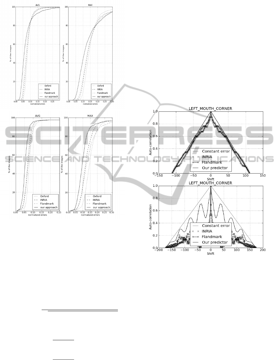
Figure 5: Cumulative distribution of point to point error

measure on the PUT and MUCT test set.

The auto-correlation vector ACor was calculated,

using function Cor, as follows. x and y are two vec-

tors and N = Card(x) = Card(y), the cardinality of

x and y. s is the shift index. Therefore, ACor(x) =

(Cor(x, x)

)

s∈[[1−N;N−1]]

Cor(x, y)



Cor

(x, y)

s ∈ A = [[0, N − 1]]

Cor

(x, y)

s ∈ B = [[1 − N, −1]]

where

Cor

(x, y)

∑

N−s

i=0

i+s

− ¯x

)(y

− ¯y

)

∑

i=0

− ¯x

)

∑

i=0

− ¯y

)

and

¯x

2 ∗ N − s

N−s

∑

i=0

i+s

¯y

2 ∗ N − s

N−s

∑

i=0

Similarly:

Cor

(x, y)

= Cor

(y, x)

−s

5.2 Results

In the two graphs represented in ﬁgure 6, we plot the

auto-correlation of a constant error vector (as a base-

line) and the normalized errors vector computed by

three different detectors. The more stable a detector

is, the closer to the baseline the corresponding curves

should be.

We present here the results for two types of video

streams: one with a speaker (whose head and lips are

moving) and another with a quiet listener (who re-

mains still). In each case, we show the graph corre-

sponding to the left corner of mouth landmark error.

The results show that our system has a better stability

Figure 6: Auto-correlation of the normalized error vector of

a non-speaking video sequence (upper graph) and a speak-

ing one (lower graph).

compared to the others in both types of video streams.

The curve oscillations observed in the lower graph

of ﬁgure 6 are due to a repetitive movement of the

speaker lips. In the upper graph, the described fea-

ture does not have a repetitive pattern. This behavior

can be regarded as an illustration of the superiority of

regression techniques over optimization based tech-

niques.

6 CONCLUSIONS

We have presented a technique of cascaded regression

for direct prediction of facial landmarks. The algo-

rithm consists of predicting successive 2D locations

VISAPP2013-InternationalConferenceonComputerVisionTheoryandApplications

518

of the landmarks in a coarse to ﬁne manner using a

series of cascaded predictors, conferring robustness to

the approach. Indeed predicting landmarks indepen-

dently results in high precision since failure to ﬁnd the

good location of one of the landmarks does not prop-

agate to the others. The regressors at each level of the

cascade are based on gradient boosting. Three kinds

of weak regressors have been assessed: linear regres-

sors, non-parametric regressors and regression trees.

The gradient boosted trees have the best performance.

This simple scheme has proved to be very efﬁcient

compared to other tested approaches in terms of loca-

tion errors. This approach is also very fast: it takes

8 milliseconds to compute the locations of 20 land-

marks (not counting the computation of the integral

image which is typically required for the detection of

the face).

As possible extensions of the approach, we could

consider applying a post-processing to the predicted

landmarks by enforcing shape consistency (Bel-

humeur et al., 2011). An attractive capability of our

model is to make it possible to trade precision against

speed by traversing only a suitable number of levels

of the cascade.

We believe that this generic approach could be ap-

plied to other problems involving regression where

features derive from measurements from the signal

e.g., to detection and localization of more generic ob-

jects using part based models.

ACKNOWLEDGEMENTS

This work was partially funded by the QUAERO

project supported by OSEO and by the European in-

tegrated project AXES.

REFERENCES

Belhumeur, P. N., Jacobs, D. W., Kriegman, D. J., and Ku-

mar, N. (2011). Localizing parts of faces using a con-

sensus of exemplars. In The 24th IEEE Conference on

Computer Vision and Pattern Recognition (CVPR).

Cao, X., Wei, Y., Wen, F., and Sun, J. (2012). Face aligne-

ment by explicit shape regression - to appear. In Proc.

of CVPR’12.

Cootes, T. F., Edwards, G. J., and Taylor, C. J. (2001). Ac-

tive appearance models. IEEE Transactions Pattern

Analysis and Machine Intelligence, 23(6):681–685.

Cootes, T. F., Taylor, C. J., Cooper, D. H., and Graham, J.

(1995). Active shape models – their training and ap-

plication. Computer Vision and Image Understanding,

61(1):38–59.

Cristinacce, D. and Cootes, T. (2008). Automatic feature

localisation with constrained local models. Pattern

Recognition, 41(10):3054–3067.

Dantone, M., Gall, J., Fanelli, G., and Van Gool, L. (2012).

Real-time facial feature detection using conditional

regression forests. In Computer Vision and Pattern

Recognition (CVPR).

Doll

ar, P., Welinder, P., and Perona, P. (2010). Cascaded

pose regression. In Computer Vision and Pattern

Recognition (CVPR), pages 1078–1085.

Everingham, M., Sivic, J., and Zisserman, A. (2006). Hello!

my name is. . . Buffy – Automatic naming of charac-

ters in TV video. In Proceedings of the British Ma-

chine Vision Conference, volume 2.

Friedman, J. H. (2001). Greedy function approximation:

A gradient boosting machine. Annals of Statistics,

29(5):1189–1232.

Jesorsky, O., Kirchberg, K. J., and Frischholz, R. (2001).

Robust Face Detection using the Hausdorff distance.

In AVBPA, pages 90–95.

Kasi

nski, A., Florek, A., and Schmidt, A. (2008). The PUT

face database. Image Processing and Communica-

tions, 13(3):59–64.

Kass, M., Witkin, A., and Terzopoulos, D. (1988). Snakes:

Active contour models. International Journal of Com-

puter Vision, 1(4):321–331.

Lanitis, A., Taylor, C. J., and Cootes, T. F. (1997). Auto-

matic interpretation and coding of face images using

ﬂexible models. IEEE Transactions Pattern Analysis

and Machine Intelligence, 19(7):743–756.

Milborrow, S., Morkel, J., and Nicolls, F. (2010). The

MUCT Landmarked Face Database. Pattern Recog-

nition Association of South Africa.

r, M., Franc, V., and Hlav

c, V. (2012). Detector of

facial landmarks learned by the structured output svm.

In Proceedings of the 7th International Conference on

Computer Vision Theory and Applications. VISAPP

’12.

Valstar, M., Martinez, B., Binefa, X., and Pantic, M. (2010).

Facial point detection using boosted regression and

graph models. In Proceedings of IEEE Int’l Conf.

Computer Vision and Pattern Recognition (CVPR’10),

pages 2729–2736, San Francisco, USA.

Viola, P. A. and Jones, M. J. (2001). Rapid object detection

using a boosted cascade of simple features. In Com-

puter Vision and Pattern Recognition (CVPR), pages

511–518.

Vukadinovic, D. and Pantic, M. (2005). Fully automatic fa-

cial feature point detection using gabor feature based

boosted classiﬁers. In Proceedings of IEEE Int’l

Conf. Systems, Man and Cybernetics (SMC’05), pages

1692–1698, Waikoloa, Hawaii.

FacialLandmarksLocalizationEstimationbyCascadedBoostedRegression

519