Efﬁcient Bag of Scenes Analysis for Image Categorization

ebastien Paris

, Xanadu Halkias

and Herv

e Glotin

2,3

DYNI team, LSIS CNRS UMR 7296, Aix-Marseille University, Aix-en-Provence, France

DYNI team, LSIS CNRS UMR 7296, Universit

e Sud Toulon-Var, Toulon, France

Institut Universitaire de France, Paris, France

Keywords:

Image Categorization, Scenes Categorization, Fine-grained Visual Categorization, Non-parametric Local

Patterns, Multi-scale LBP/LTP, Dictionary Learning, Sparse Coding, LASSO, Max-pooling, SPM, Linear

SVM.

Abstract:

In this paper, we address the general problem of image/object categorization with a novel approach referred to

as Bag-of-Scenes (BoS).Our approach is efﬁcient for low semantic applications such as texture classiﬁcation

as well as for higher semantic tasks such as natural scenes recognition or ﬁne-grained visual categorization

(FGVC). It is based on the widely used combination of i) Sparse coding (Sc), ii) Max-pooling and iii) Spa-

tial Pyramid Matching (SPM) techniques applied to histograms of multi-scale Local Binary/Ternary Patterns

(LBP/LTP) and its improved variants. This approach can be considered as a two-layer hierarchical architec-

ture: the ﬁrst layer encodes the local spatial patch structure via histograms of LBP/LTP while the second en-

codes the relationships between pre-analyzed LBP/LTP-scenes/objects. Our method outperforms SIFT-based

approaches using Sc techniques and can be trained efﬁciently with a simple linear SVM.

1 INTRODUCTION

Image categorization

consists of assigning a unique

label with a generally high-level semantic value to

an image while FGVC refers to the task of classify-

ing objects that belong to the same basic-level class.

Both have long been a challenging problem area in

computer vision, biomonitoring and robotics and can

mainly be viewed as belonging to the broader super-

vised classiﬁcation framework. In scene categoriza-

tion, the difﬁculty of the task can be partly explained

by the high-dimensional input space of the images as

well as the high-level semantic visual concepts that

lead to large intra-class variation. For object recog-

nition more speciﬁcally, the small aspect ratio (ob-

ject’size vs image’size) can induce a high level of un-

informative background pixels. A preliminary detec-

tion procedure is required to ”home-in” the object in

a Region of Interest (ROI) (Bosch et al., 2007; Larios

et al., 2011).

The direct framework (see Fig.1) in vision sys-

tems consists of extracting directly from the images

meaningful features (using shape/texture/similarity/

color information) in order to achieve the maximum

Granded by COGNILEGO ANR 2010-CORD-013 and

PEPS RUPTURE Scale Swarm Vision

generalization capacity during the classiﬁcation stage.

Examples of such popular features in computer vision

and human cognition inspired models include GIST

(Oliva and Torralba, 2001), HOG (Dalal and Triggs,

2005), Self-Similarity (Deselaers and Ferrari, 2010)

and WLD (Chen et al., 2010).

Widely used in face detection (Fr

oba and Ernst,

2004; Wu et al., 2011), face recognition (Marcel et al.,

2007; Zhang et al., 2007), texture classiﬁcation (Sa-

dat et al., 2011; Bianconi et al., 2012) and scene cat-

egorization (Wu and Rehg, 2008; Gao et al., 2010;

Paris and Glotin, 2010; Zhang et al., 2010), Local

Binary Pattern (LBP) (Ojala et al., 2002) and re-

cent derivatives such as Local Ternary Pattern (LTP)

(Zheng et al., 2010), Gabor-LBP (Zhang et al., 2009;

Lee et al., 2010), Local Gradient Pattern (LGP) (Jun

and Kim, 2012) or Local Quantized Pattern (LQP)

(Hussain and Triggs, 2012) are efﬁcient local micro-

patterns that deﬁne competitive features achieving

state-of-the-art performances.

LBP can be considered as a non-parametric local

visual micro-pattern texture, encoding mainly con-

tours and differential excitation information of the 8

neighbors surrounding a central pixel (Heikkil

a et al.,

2006; Huang et al., 2011). This process represents

a contractive mapping from R

7→ N

⊂ N

for

335

Paris S., Halkias X. and Glotin H. (2013).

Efﬁcient Bag of Scenes Analysis for Image Categorization.

In Proceedings of the 2nd International Conference on Pattern Recognition Applications and Methods, pages 335-344

DOI: 10.5220/0004198303350344

 SciTePress

each local patch p(x

x) centered in x

x ((Bianconi and

Fern

andez, 2011) provide a theoretical study of LBP).

The total number of different LBPs is relatively small

and by construction is ﬁnite: from 256 up to 512 dif-

ferent patterns (if improved LBP is used).

LTP (Tan and Triggs, 2010) have been extended

from LBP as a parametric approximation of a ternary

pattern. Instead of mapping R

7→ N

⊂ N

, they

proposed to split the ternary pattern into two binary

patterns and concatenating the two associated his-

tograms. In (Hussain and Triggs, 2012), they general-

ize local pattern with LQP by both increasing neigh-

borhood range, number of neighbors and pattern car-

dinality leading to map R

7→ N

⊂ N

Histograms of LBP (HLBP) (respectively HLTP),

which count the occurrence of each LBP (respectively

LTP) in the scene, can easily capture general struc-

tures in the visual scene by integrating information

in a ROI, while being less sensitive to local high fre-

quency details. This property is important when the

desire is to generalize visual concepts. As depicted in

this work, it is advantageous to extend this analysis

for several sizes of local ROIs using a spatial pyramid

denoted by Λ

Λ.

Recently, the alternative scheme of Bag-of-

Features (BoF) has been employed in several com-

puter vision tasks with wide success. It offers a deeper

extraction of visual concepts and improves accuracy

of computer vision systems. BoF image representa-

tion (Willamowski et al., 2004) and its SPM exten-

sion (Lazebnik et al., 2006) share the same idea as

HLBP: counting the presence (or combination) of vi-

sual patterns in the scene. BoF contains at least three

modules prior to the classiﬁcation stage: (i) region se-

lection for patch extraction; (ii) codebook/dictionary

generation and feature quantization; (iii) frequency

histogram based image representation with SPM. In

general, SIFT/HOG patches (Lowe, 2009; Dalal and

Triggs, 2005) are employed in the ﬁrst module. These

visual descriptors are then encoded, in an unsuper-

vised manner, into a moderate sized dictionary using

Vector Quantization (VQ) (Lazebnik et al., 2006) or

sparse coding (Yang et al., 2009b). In (Wu and Rehg,

2009), Wu and al were ﬁrst to introduce LBP (via

CENTRIST) into BoF framework coupled with his-

togram intersection kernel (HIK).

At least two disadvantages can be addressed

against the BoF framework, mainly concerning the

second stage. Firstly, and more speciﬁcally for

FGVC, the trained dictionaries don’t have enough

representative basis vectors for some (rare and de-

tailed) local patches that are crucial for discrimina-

tivity. Secondly, during quantiﬁcation/encoding a lot

of important information can be lost (Boiman et al.,

2008). For these reasons, dictionary-free approaches

have been recently introduced. In (Yao and Bradski,

2012), they performed an efﬁcient template matching

coupled with a bagging classiﬁcation procedure. In

(Bo et al., 2010; Bo et al., 2011a), they bypass BoF

with efﬁcient but computationally expensive hierar-

chical kernel descriptors. In (Larios et al., 2011; Choi

et al., 2012), they proposed patche’s supervised learn-

ing (respectively supervised projection) with random

forest (respectively with PLS).

In order to improve the encoding scheme, it has

been shown that localized soft-assignement (Avila

et al., 2011), local-constrained linear coding (LLC)

(Oliveira et al., 2012), Fisher vectors (FV) (Perronnin

et al., ; Krapac et al., 2011), orthogonal matching pur-

suit (OMP) (Bo et al., 2011b) or Sparse coding (Sc)

(Yang et al., 2009b; Gao et al., 2010) can easily be

plugged into the BoF framework as a replacement for

VQ. Moreover, pooling techniques coupled with SPM

(Lazebnik et al., 2006) can be effectively used as a re-

placement for the global histogram based image rep-

resentation.

Our contributions in this paper are two-fold. We

ﬁrst re-introduce two multi-scale variants of the LBP

operators and extend two novel multi-scale variants

of the LTP operators (Tan and Triggs, 2010). Sec-

ondly, we propose to plug HLBP/HLTP into the Sc

framework as a second analyzing layer and call this

procedure Bag-of-Scenes (BoS). This new approach

is efﬁcient as well as for scene categorization, ob-

ject recognition or FGVC. The novel features can

be trained efﬁciently with simple large-scale linear

SVM solver such as Pegasos (Shalev-Shwartz et al.,

2007) or LIBLINEAR (Hsieh et al., 2008). BoS can be

seen as a two layer Hierarchical BoF analysis: a ﬁrst

fast contractive low-dimension manifold encoder via

HLBP/HLTP and a second inﬂating high-dimension

encoder via Sc.

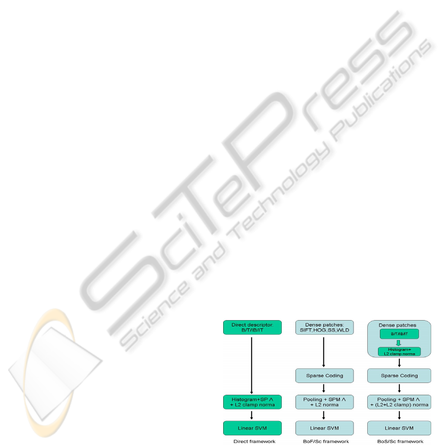
Figure 1: Comparison of the different frameworks. Left:

direct framework, Middle: BoF/Sc framework, Right: Our

proposed BoS/Sc framework.

ICPRAM2013-InternationalConferenceonPatternRecognitionApplicationsandMethods

336

2 HISTOGRAM OF

MULTI-SCALE LOCAL

PATTERNS

For an image/patch I

I (n

× n

), we present two exist-

ing multi-scale versions of the LBP operator, denoted

by the B operator and for its improved variant by the

IB operator. We also introduce two novel multi-scale

versions of the LTP, denoted by the T operator and for

its improved variant by the IT operator.

2.1 Multi-scale LBP/ILBP

Basically, operator B encodes the relationship be-

tween a central block of (s × s) pixels located in

) with its 8 neighboring blocks (Liao et al.,

2007), whereas operator IB adds a ninth bit encod-

ing a term homogeneous to the differential excitation

(see left Fig. 2). Both can be considered as a non-

parametric local texture encoder for scale s. In order

to capture information at different scales, the range

analysis s ∈ S , is typically set at S = [1,2,3,4] for this

paper, where S = Card(S ). These two micro-codes

are deﬁned as follows











B(y

,s) =

i=7

∑

i=0

≥A

}

IB(y

,s) = B(y

,s) + 2



∑

i=0

≥8Ac



(1)

For ∀(y

) ∈ R

R ⊂ I

I, B(y

,s) ∈ N

and

IB(y

,s) ∈ N

respectively.

Figure 2: Left: I

I and B(y

,4) overlaid. Right: corre-

sponding image integral I

I and the central block A

. A

can

be efﬁciently computed with the 4 corner points.

2.2 Multi-scale LTP/ILTP

We introduce the multi-scale version of LTP and its

improved variant. The idea behind LTP is to extend

the LBP for b = 3 with the help of a single thresh-

old parameter t ∈ N

. With the same neighborhood

{x}

= 1 if event x is true, 0 otherwise.

conﬁguration with N = 8 (see left Fig. 2), a direct

extension would conduct to have 3

= 6561 different

patterns. In (Tan and Triggs, 2010), they proposed to

break the high dimensionality of the code by splitting

the ternary code into two binary operators T

and T

such as:











,s;t) =

i=7

∑

i=0

{

−A

)≥t}

,s;t) =

i=7

∑

i=0

{

−A

)≤−t}

(2)

The improved multi-scale LTP operators (denoted IT

and IT

) are derived similarly from MSLBP by:











,s;t) = T

,s;t) + 2





∑

i=0

−8Ac



≥t



,s;t) = T

,s;t) + 2





∑

i=0

−8Ac



≤−t



(3)

Now, for ∀(y

) ∈ R

R ⊂ I

I, both codes

,s;t),T

,s;t)} ∈ N

while the im-

proved version {IT

,s;t),IT

,s;t)} ∈ N

respectively.

2.3 Integral Image for Fast Areas

Computation

The different areas {A

} and A

in eq.(1), eq.(2) and

eq.(3) can be computed efﬁciently using the image in-

tegral technique (Viola and Jones, 2004). Let’s deﬁne

I the image integral of I

I by:

I(y, x) ,

∑

I(y

). (4)

Any square area A(y,x,s) ∈ R

R (see right Fig. 2) with

upper-left corner located in (y,x) and side length s is

the addition of only 4 values:

A(y, x, s) = I

I(y + s,x + s) + I

I(y, x)

−(I

I(y, x + s) + I

I(y + s,x)).

(5)

2.4 Histogram of Local Patterns

For all previously deﬁned operators op ∈

{B,IB,T

,IT

}, efﬁcient features are ob-

tained by counting occurrences of the j

visual

LBP/LTP at scale s in a ROI R

R ⊆ I

R, j,s) =

∑

)∈R

{op(y

,s)= j}

where j = 0,...,b − 1 is the j

bin of the his-

togram and b = {256,512,256,256,512,512} for

op ∈ {B, IB, T

,IT

} respectively.

EfficientBagofScenesAnalysisforImageCategorization

337

Full histogram of LBP and variant its ILBP, de-

noted z

, z

, are computed by:

R,s) , [z

R,0,s),...,z

R,b − 1,s)], (6)

with a total size for patches d = b = {256, 512} re-

spectively.

For LTP, full histograms, denoted z

, z

are de-

ﬁned by:

R,s) ,



R,0,s),...,z

R,b − 1,s),...,

,...,z

R,0,s),...,z

R,b − 1,s)],

(7)

with a total size for patches d = 2.b = {512, 1024}

respectively.

To end the patch extraction stage, regardless the

type of histogram of local patterns used, a `

clamped

normalization procedure (`

normalization followed

by a saturation with the clamp value and again a

normalization) is performed on each histogram

(clamp value = 0.2).

3 SPARSE CODING ON PATCHES

OF MULTI-SCALE LOCAL

PATTERNS

Following the same framework as in (Lazebnik et al.,

2006; Yang et al., 2009b; Boureau et al., 2010a; Chat-

ﬁeld et al., 2011), we show here that the traditional

BoF approach can be advantageously replaced by i)

Sc, ii) max-pooling technique and iii) a simple linear

SVM as a classiﬁer since the produced features are

mostly linearly separable (see Fig. 1 for synopsis).

3.1 Patches of HB/HIB/HT/HIT

Here, we replace the collection of usual SIFT patches

densely sampled on a grid by our HB/HIB/HT/HIT

patches z

z seen previously. Speciﬁcally, F patches of

size (m × m) associated with ROI’s {O

} (possibly

overlapping) are extracted for k = 0,...,F − 1 and

∀s ∈ S (see Fig. 3). For a faster computation for each

scale s, the integral image I

I is ﬁrst computed from I

For a complete dataset containing N images and

∀s ∈ S, we obtain a collection of P = TS patches

Z , {z

}, i = 1, . . . , P, where T = NF. We deﬁne,

the subset of patches z

at scale s by Z

Z(s) ⊆ Z

Z with T

elements.

3.2 Sparse Coding Overview

In order to obtain highly discriminative visual fea-

tures, a common procedure consists of encoding each

patch z

∈ Z

Z(s) at scale s through an unsupervised

trained dictionary D

D , [d

,. .. , d

] ∈ R

b×K

, where K

denotes the number of dictionary elements, and its

corresponding weight vector c

∈ R

. In the BoF

framework, the vector c

is assumed to have only one

non-zero element:

argmin

D,C

∑

i=1

− D

s.t. kc

= 1, (8)

where C

C , [c

,. .. , c

] and k • k

deﬁnes the pseudo

zero-norm, where here only one element of c

is non-

zero. In eq. (8), under these constraints, (D

D,C

C) can be

optimized jointly by a Kmeans algorithm for example.

In the Sc approach, in order to i) reduce the quan-

tization error and ii) to have a more accurate represen-

tation of the patches, each vector z

is now expressed

as a linear combination of a few vectors of the dic-

tionary D

D and not only by a single one. Imposing

the exact number of non-zero elements in c

(spar-

sity level) involves a non-convex optimization (Mairal

et al., 2009). In general, it is preferred to relax this

constraint and to use instead an `

penalty which also

involves sparsity. The problem is then reformulated

using the following equation:

argmin

D,C

∑

i=1

− D

+ βkc

s.t. kc

= 1,

(9)

where the sparsity in controlled by the parameter β.

The last equation is not jointly convex in (D

D,C

C) and

a common procedure consists of optimizing alterna-

tively D

D given C

C by a block coordinate descent and

then C

C given D

D by a LASSO procedure (Tibshirani,

1996). At the end of the process, for each scale s ∈ S ,

a trained dictionary

D(s) is obtained.

3.3 Spatial Pyramidal Matching

and Max Pooling

For an image I

I and given a trained dictionary

D(s)

for a type of code at scale s, F sparse vectors {c

(s)}

are computed by a LASSO algorithm. The ﬁnal

efﬁcient descriptor x

x(s) ,



(s),. . . , x

K−1

(s)



∈ R

is obtained by the following max-pooling procedure

(Yang et al., 2009b; Boureau et al., 2010b):

(s) , max

k|O

∈R

(|c

(s)|), j = 0,...,K − 1, (10)

where each element of x

x(s) represents the max-

response of the absolute value of sparse codes belong-

ing to the ROI R

R. In order to improve accuracy, a spa-

tial pyramidal matching procedure helps to perform

a more robust local analysis. The spatial pyramid

Λ has V =

L−1

∑

l=0

ROIs {R

l,v

} with l = 0, . . . , L − 1,

ICPRAM2013-InternationalConferenceonPatternRecognitionApplicationsandMethods

338

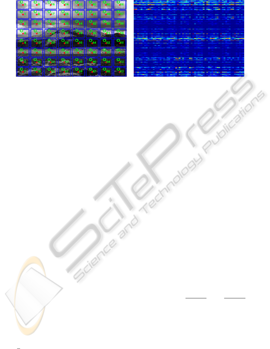
Figure 3: Example Left: ROI’s {O

}, k = 0, . . ., F −1 of extracted patches used to compute HB. Right: associated normalized

histograms {z

)}, one per column.

v = 0, . . . ,V

− 1 (see Fig. 4 for an example). The

quantity z

l,v

(s) for each ROI R

l,v

is computed by:

l,v

(s) , max

k|O

∈R

l,v

(|c

(s)|), j = 0,...,K − 1. (11)

We reinforce our model by an important normal-

ization step, improving considerably accuracy, con-

sists of the `

normalization of all vectors {x

l,v

(s)},

v = 0,. . . ,V

− 1,s ∈ S , i.e. belonging to the same

pyramidal layer l. This step is also very important

and often hidden in the existing literature.

The ﬁnal descriptor x

x(Λ

Λ) will be deﬁned by the

weighted concatenation of all the x

l,v

(s) vectors, i.e.

x(Λ

Λ) , {λ

l,v

(s)}, l = 0,. . . , L − 1, v = 0, . . . ,V

− 1

and ∀s ∈ S . The total size of the feature vector x

x(Λ

Λ)

is d = K.V.S, where typically in our simulations, we

ﬁxed K = {1024, 2048}, V = {10,21, 26} and S = 4.

A ﬁnal `

clamped normalization step is performed on

the full vector x

x(Λ

Λ).

4 LINEAR SVM FOR

SUPERVISED TRAINING

Let’s assume available a training data set

(Λ

Λ),y

}

i=1

, where x

(Λ

Λ) ∈ R

is one of four

previously deﬁned features and y

∈ {1, . . . , M},

where M is the number of classes. As in (Yang

et al., 2009b; Boureau et al., 2010a), we will use a

simple large-scale linear SVM such as LIBLINEAR

(Hsieh et al., 2008) with the 1-vs-all multi-class

strategy. The associated binary unconstrained convex

optimization problem to solve is:

min

(

w +C

∑

i=1

max



1 − y



)

, (12)

where the parameter C controls the generalization er-

ror and is tuned on a speciﬁc validation set. LIBLIN-

EAR converges to a solution linearly in O(dN) com-

pared to O(dN

) in the worst case for classic SVM

where N

≤ N deﬁnes the number of support vectors.

5 EXPERIMENTAL RESULTS

We test our BoS framework on Scene-15 (Lazeb-

nik et al., 2006), UIUC-Sport (Li, 2007), Caltech101

(Fei-Fei et al., 2007), USCD-Birds200 (Welinder

et al., 2010) and Stanford-Dogs120 datasets(Khosla

et al., 2011a).

We deﬁne our SPM matrix Λ

Λ with L levels such

as Λ

Λ , [r

,λ

λ]. Λ

Λ is matrix of size (L × 5).

For a level l ∈ {0, . . . , L − 1}, the image I

I, with size

× n

), is divided into potentially overlapping sub-

windows R

l,v

of size (h

×w

). All these windows are

sharing the same associated weight λ

. In our imple-

mentation, h

, bn

y,l

c and w

, bn

x,l

c where r

y,l

x,l

and λ

are the l

element of vectors r

, r

and λ

respectively. Sub-window shifts in x − y axis are de-

ﬁned by integers δ

y,l

, bn

y,l

c and δ

x,l

, bn

x,l

where d

y,l

and d

x,l

are elements of d

and d

respec-

tively. Overlapping can be performed if d

y,l

≤ r

y,l

and/or d

x,l

≤ r

x,l

. The total number of sub-windows is

equal to

V =

L−1

∑

l=0

L−1

∑

l=0

(1 − r

y,l

)

y,l

+ 1c.b

(1 − r

x,l

)

x,l

+ 1c.

(13)

For all dataset used, we used SIFT patches

with block size (16 × 16) pixels and (26 × 26)

pixels for ours HB/HIB/HT/HIT respectively. For

SIFT/HB/HIB/HT/HIT, we extract F = 35.35 = 1225

patches per scale. For both dictionary learning and

sparse codes computation, we ﬁx β = 0.2 and N

ite

50 iterations to train dictionaries. We uses our own

modiﬁed version of the SPAMS toolbox (Mairal et al.,

2009). Finally, we performed 10 cross-validation to

EfficientBagofScenesAnalysisforImageCategorization

339

Figure 4: Example of SPM Λ

Λ with L = 3, F = 8 × 8 and V = 1 + 4 + 16. The F ROIs {O

}, k = 0,. . . , F − 1 associated with

each patch z

are represented by blue squares. Sparse codes c

are computed for each ROI O

. Upper-left corner of each max-

pooling window R

l,v

taking {64, 16, 4} c

is indicated with a green cross. Left: R

0,0

= I

I for l = 0. Middle: {R

1,v

}, v = 0, . .. , 3

for l = 1. Right {R

2,v

}, v = 0,. .. , 15 for l = 2.

compute the average overall accuracy and its standard

deviation using the LIBLINEAR solver and ﬁxing pa-

rameter C = 15.

5.1 Scene-15 Dataset

The Scene-15 dataset contains a total of 4485 im-

ages in grey color assigned to M = 15 categories.

The number of images in each category is ranging

from 200 to 400. 100 images per class are used to

train, the rest for testing. For this dataset, we de-

ﬁne Λ

Λ =



1 1 1 1 1



, i.e. a two layer spa-

tial pyramid dividing image in third and an overlap-

ping of 50% representing a total of 1 + 25 = 26 ROIs.

For HT and HIT patches, we ﬁx t = 1. We select

15000 patches per class (a total of 225000 patches)

to train dictionaries via Sc. In Fig. 5, we plot ac-

curacy versus the number of words K in the dictio-

nary training. With our particular choice of Λ

Λ and

for one unique scale, we retrieved results comparable

to (Yang et al., 2009b), i.e. 80.28% vs. 81.24% for

our implementation. Whatever, the number of scale

used and the type of patch, our BoS framework out-

performs the SIFT-ScSPM approach. In Tab. 1, we

compare our results with the state-of-the-art for this

dataset (with S = 4 scales). The best performance is

actually obtained with the SIFT-LScSPM involving

a more sophisticated dictionary training through the

Laplacian sparse coding. The latter is very time and

memory consuming

but is improving results with

normal SIFT patches from 80.28% ± 0.93 with sim-

ple Sc to 89.75% ± 0.5 with LSc. The second best

result is obtained with spatial FV following by the

kernel descriptors. For FV, they reduced SIFT to 64

LSc requiers to store sparse codes of the template set,

i.e, a sparse matrix (K × N

template

dimension (total size equal to K(1 + 2.d) = 12800)

and used a multi-class logistic regression. It is also

worth noting that KDES-EKM uses a concatenation

of 3 descriptors coupled with an efﬁcient feature map-

ping (KDES-A+LSVM got 81.9% ± 0.60 for a fair

comparison). However, our results with a single HIT

patch and a simple linear SVM are very close. More,

if FV or LSc would be used, one can expect better

results.

Table 1: Recognition rate (and standard deviation) for

Scene-15 dataset.

Algorithms Accuracy ± Std

SIFT-ScSPM (K = 1024) (Yang et al., 2009b) 80.28% ± 0.93

SIFT-MidLevel (K = 2048) (Boureau et al., 2010a) 84.20% ± 0.30

SIFT-LScSPM (K = 1024) (Gao et al., 2010) 89.75% ± 0.50

KDES-EKM (K = 1000) (Bo et al., 2010) 86.70%

PCASIFT-SFV (K = 100) (Krapac et al., 2011) 88.20%

SIFT-DITC (K = 1000) (Elﬁky et al., 2012) 85.4%

SIFT-ScSPM (K = 1024, our implementation) 81.24% ± 0.73

HB-ScSPM (K = 2048, our work) 86.04%±0.36

HIB-ScSPM (K = 2048, our work) 86.45%±0.44

HT-ScSPM (K = 2048, our work) 86.24%±0.43

HIT-ScSPM (K = 2048, our work) 86.53% ± 0.37

5.2 UIUC-sport Dataset

The UIUC-sport dataset contains a total of 1579 im-

ages assigned to M = 8 categories. 60 images per

class are used to train, 70 for testing. For this dataset,

we deﬁne Λ

Λ =



1 1 1 1 1



representing a

total of 1 + 9 = 10 ROIs for SPM. Color (R,G,B) in-

formation channels are used, sampling patches and

training dictionaries on each of them. For HT and

HIT patches, we ﬁx t = 5. We select 30000 patches

per class (a total of 240000 patches) to train dictio-

naries via Sc. In Fig. 6, we plot accuracy vs. K. No-

ICPRAM2013-InternationalConferenceonPatternRecognitionApplicationsandMethods

340

128 256 512 1024 2048

0.75

0.76

0.77

0.78

0.79

0.8

0.81

0.82

0.83

0.84

# K

Accuracy

Scenes15 with one scale

SIFT−ScSPM, σ=[1]

HB−ScSPM, s=[1]

HIB−ScSPM, s=[1]

HT−ScSPM, s=[1]

HIT−ScSPM, s=[1]

128 256 512 1024 2048

0.78

0.79

0.8

0.81

0.82

0.83

0.84

0.85

0.86

0.87

# K

Accuracy

Scenes15 with four scales

SIFT−ScSPM, σ=[0.5,0.65,0.8,1]

HB−ScSPM, s=[1,2,3,4]

HIB−ScSPM, s=[1,2,3,4]

HT−ScSPM, s=[1,2,3,4]

HIT−ScSPM, s=[1,2,3,4]

Figure 5: Results for Scenes 15. Left: one scale are used for all kind of patches. Right: four scales are used for all kind of

patches.

128 256 512 1024 2048

0.8

0.81

0.82

0.83

0.84

0.85

0.86

0.87

0.88

0.89

# K

Accuracy

UIUC−Sport with one scale

SIFT−ScSPM, σ=[1]

HB−ScSPM, s=[1]

HIB−ScSPM, s=[1]

HT−ScSPM, s=[1]

HIT−ScSPM, s=[1]

128 256 512 1024 2048

0.84

0.85

0.86

0.87

0.88

0.89

0.9

# K

Accuracy

UIUC−Sport with four scales

SIFT−ScSPM, σ=[0.5,0.65,0.8,1]

HB−ScSPM, s=[1,2,3,4]

HIB−ScSPM, s=[1,2,3,4]

HT−ScSPM, s=[1,2,3,4]

HIT−ScSPM, s=[1,2,3,4]

Figure 6: Results for UIUC-Sport. Left: one scale are used for all kind of patches. Right: four scales are used for all kind of

patches.

tice, that our implementation of SIFT-ScSPM outper-

forms results from (Yang et al., 2009b). Our choice of

Λ, color information used in training and our speciﬁc

normalization procedure may explain these improved

results. We can also notice, especially for a small dic-

tionary size, that our BoS framework is far superior to

SIFT-ScSPM. In Tab. 2, we compare our results with

the state-of-the-art (with S = 4 scales). To our best of

knowledge, our BoS framework, with HIT patch, ob-

tains the state-of-the-art performances with 89.85%

of overall accuracy.

5.3 Caltech101 Dataset

The Caltech101 dataset contains a total of 9144 im-

ages assigned to M = 102 categories. 30 images per

class are used to train, the rest for testing. For this

dataset, we deﬁne Λ

Λ =



1 1 1 1 1



. We ex-

tract 2000 HIT patches per class (a total of 204000

patches) for S = 4 scales to train dictionaries via Sc.

Table 2: Recognition rate (and standard deviation) for

UIUC-Sport dataset.

Algorithms Accuracy ± Std

SIFT-ScSPM (K = 1024) (Yang et al., 2009b) 82.70% ± 1.50

SIFT-LScSPM (K = 1024) (Gao et al., 2010) 85.30% ± 0.31

SIFT-HOMP (K = 2 × 1024) (Bo et al., 2011b) 85.70% ± 1.30

SIFT-ScSPM (K = 1024, our implementation) 87.98% ± 1.08

HB-ScSPM (K = 2048, our work) 87.42%±1.27

HIB-ScSPM (K = 2048, our work) 88.44%±1.25

HT-ScSPM (K = 2048, our work) 89.35%±1.42

HIT-ScSPM (K = 2048, our work) 89.85% ± 1.28

In Tab. 3, we compare our results with the state-of-

the-art. We separate methods using more sophisti-

cated approaches such as prior detection to localize

more precisely objects or using complex supervised

segmentation with methods classifying directly im-

ages. To the best of our knowledge, we have the

highest recognition rate (81.05%) for a unique feature

coupled with a simple linear SVM. With a medium

dictionary size (K = 1024), we are competitive with

sophisticated and time-consuming methods using su-

EfficientBagofScenesAnalysisforImageCategorization

341

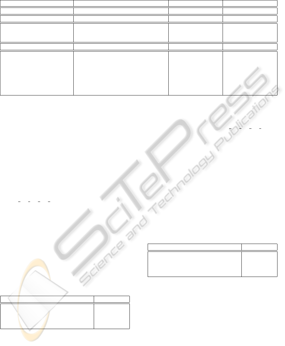
Table 3: Recognition rate (and standard deviation) for Caltech101 dataset.

Methods Algorithms Accuracy ± Std (15 Train) Accuracy ± Std (30 Train)

Graph Matching + SVM. MLMRF+Curv. Expen. (Duchenne et al., 2011) 75.30% ± 0.70 80.30% ± 1.20

Detec. + Mult Non-Lin Ker. Multiway-SVM (Bosch et al., 2007) - 81.30%

Superv. Segm+Classif Subcat. Relevances (Todorovic and Ahuja, 2008) 72.00% 82.00%

Superv. Segm+Classif+Non-Lin Ker SvcSegm (Li et al., 2010) 72.60% 79.20%

Superv. Segm+Regress+Non-Lin Ker SvrSegm (Li et al., 2010) 74.70% 82.30%

Classif+MKL GS-MKL (Yang et al., 2009a) 73.20% 84.30%

Classif+Lin Ker SIFT-Multiway (K = 1024) (Boureau et al., 2011) - 77.30%± 0.60

Classif+Lin Ker SIFT-CDBN (K = 4096) (Sohn et al., 2011) 71.30% 77.80%

Classif+Non-Lin Ker SIFT-LaRank (K = 4096) (Oliveira et al., 2012) 73.09% ± 0.77 80.02% ± 0.36

Classif+Lin Ker HT-ScSPM (K = 1024, our work) 74.24% ± 0.69 81.05% ± 0.43

Classif+Lin Ker HT-ScSPM (K = 2048, our work) 73.92% ± 0.81 80.90% ± 0.38

Classif+Lin Ker HIT-ScSPM (K = 1024, our work) 73.23% ± 0.69 80.51% ± 0.46

Classif+Lin Ker HIT-ScSPM (K = 2048, our work) 72.54% ± 0.70 80.27% ± 0.44

pervised segmentation, graph matching or complex

MKL.

5.4 USCD-Birds200 Dataset

The USCD-Birds200 dataset is containing a total

of 6033 images assigned to M = 200 categories.

We crop all images with the provided bounding-box

ground-truth. 15 images per class are used to train,

the rest for testing. This dataset represents a challeng-

ing FGVC task, where categorization must exploits

details difference between species. We particularize

Λ =



1 1 1 1 1



. Color (R,G,B) informa-

tion channels are used, sampling patches and training

dictionaries on each of them. For the HIT patches, we

ﬁx t = 5. We select 2000 patches per class (a total

of 400000 patches) for S = 4 scales to train dictionar-

ies via Sc. In Tab. 4, we compare our results with

the state-of-the-art. To our best of knowledge, our

BoS framework, with HIT patch, obtains the state-

of-the-art performances with 27.93% of overall accu-

racy, outperforming dictionary-free methods.

Table 4: Recognition rate and standard deviation on the

USCD-Birds200 dataset.

Algorithms Accuracy ± Std

BiCOS-MT (Chai et al., 2011) 16.20%

Discri. Decision Trees + RF (Yao et al., 2011) 19.20%

Mult.-Cue+DITC (K = 5000) (Khan et al., 2011) 22.40%

HIT-ScSPM (K = 1024, our work) 27.93% ± 1.16

5.5 Stanford-Dogs120 Dataset

The Stanford-Dogs120 dataset is containing a total

of 20580 images assigned to M = 120 categories.

We crop all images with the provided bounding-box

ground-truth. 100 images per class are used to train,

the rest for testing (we use the provided train/test

set). This dataset represents also a challenging FGVC

task. We particularize Λ

Λ =



1 1 1 1 1



Color (R,G,B) information channels are used, sam-

pling patches and training dictionaries on each of

them. For the HIT patches, we ﬁx t = 5. We select

2000 patches per class (a total of 240000 patches) for

S = 3 scales (S = {1, 2, 3}) to train dictionaries via

Sc. In Tab. 5, we compare our results with the state-

of-the-art. To our best of knowledge, our BoS frame-

work, with HIT patch, obtains the state-of-the-art per-

formances with 36.36% of overall accuracy with a

unique descriptor and linear SVM. A simple late fu-

sion of SIFT-ScSPM with HIT-ScSPM (product of

p(y = 1|x

x)) gives a score of 40.03%.

Table 5: Recognition rate and standard deviation on the

Stanford-Dogs120 dataset.

Algorithms Accuracy ± Std

SIFT-ScSPM (Khosla et al., 2011b) 26.10%

SIFT-ScSPM (K = 2048, our implementation) 32.05%

HIT-ScSPM (K = 2048, our work) 36.36%

SIFT-ScSPM+HIT-ScSPM (K = 2048, our work) 40.03%

6 CONCLUSIONS AND

PERSPECTIVES

We have presented in this article the 2-layer BoS

architecture mixing HB/HIB/HT/HIT as a fast local

textures encoder for the ﬁrst layer and Sc as scenes

encoder for the second. This ﬁrst hand-graft layer

can advantageously replace complex hierarchical fea-

ture extractors such as Deep Belief Networks and

the patch extraction are even faster than SIFT ones,

thanks to the integral image technique. Achieved

performances outperform state-of-the-art results with

ICPRAM2013-InternationalConferenceonPatternRecognitionApplicationsandMethods

342

a simple linear SVM as well for object recognition

tasks as for FGVC ones.

As potential future works, many perspectives can

be investigated. For example, complementary patch,

multi-scale variants of LPQ could be coupled with our

HB/HIB/HT/HIT approach, in order train a unique

dictionary with these fused patches. Higher dimen-

sion local pattern can be also associated with the

Sc framework such those proposed by (Hussain and

Triggs, 2012). Finally, experimenting with LSc (Gao

et al., 2010) or FV (Krapac et al., 2011) should im-

prove the encoding part of the pipeline, while super-

vised pooling techniques (Jia et al., 2011) will surely

also improve results.

REFERENCES

Avila, S. E. F., Thome, N., Cord, M., Valle, E., and de Al-

buquerque Ara

ujo, A. (2011). Bossa: Extended bow

formalism for image classiﬁcation. In ICIP’ 11.

Bianconi, F. and Fern

andez, A. (2011). On the occur-

rence probability of local binary patterns: A theoret-

ical study. Journal of Mathematical Imaging and Vi-

sion, 40(3):259–268.

Bianconi, F., Gonz

alez, E., Fern

andez, A., and Saetta,

S. A. (2012). Automatic classiﬁcation of granite tiles

through colour and texture features. Expert Syst.

Appl., 39(12):11212–11218.

Bo, L., Lai, K., Ren, X., and Fox, D. (2011a). Object recog-

nition with hierarchical kernel descriptors. In CVPR’

11.

Bo, L., Ren, X., and Fox, D. (2010). Kernel descriptors for

visual recognition. In NIPS’ 10.

Bo, L., Ren, X., and Fox, D. (2011b). Hierarchical matching

pursuit for image classiﬁcation: Architecture and fast

algorithms. In NIPS’ 11, pages 2115–2123.

Boiman, O., Shechtman, E., and Irani, M. (2008). In de-

fense of nearest-neighbor based image classiﬁcation.

In CVPR’ 08.

Bosch, A., Zisserman, A., and Munoz, X. (2007). Im-

age classiﬁcation using random forests and ferns. In

ICCV’ 07.

Boureau, Y., Bach, F., LeCun, Y., and Ponce, J. (2010a).

Learning mid-level features for recognition. In CVPR’

10.

Boureau, Y., Le Roux, N., Bach, F., Ponce, J., and LeCun,

Y. (2011). Ask the locals: multi-way local pooling for

image recognition. In ICCV’ 11.

Boureau, Y., Ponce, J., and LeCun, Y. (2010b). A theoreti-

cal analysis of feature pooling in vision algorithms. In

ICML’ 10.

Chai, Y., Lempitsky, V. S., and Zisserman, A. (2011). Bicos:

A bi-level co-segmentation method for image classiﬁ-

cation. In ICCV’ 11.

Chatﬁeld, K., Lempitsky, V., Vedaldi, A., and Zisserman,

A. (2011). The devil is in the details: an evaluation of

recent feature encoding methods. In BMVC.

Chen, J., Shan, S., He, C., Zhao, G., Pietikainen, M., Chen,

X., and Gao, W. (2010). Wld: A robust local image

descriptor. IEEE Trans. PAMI, 32(9).

Choi, J., Schwartz, W. R., Guo, H., and Davis, L. S. (2012).

A complementary local feature descriptor for face

identiﬁcation. In WACV’ 12.

Dalal, N. and Triggs, B. (2005). Histograms of oriented

gradients for human detection. In CVPR’ 05.

Deselaers, T. and Ferrari, V. (2010). Global and efﬁcient

self-similarity for object classiﬁcation and detection.

In CVPR’ 10.

Duchenne, O., Joulin, A., and Ponce, J. (2011). A graph-

matching kernel for object categorization. In ICCV’

11.

Elﬁky, N. M., Khan, F. S., van de Weijer, J., and Gonz

alez,

J. (2012). Discriminative compact pyramids for ob-

ject and scene recognition. Pattern Recognition,

45(4):1627–1636.

Fei-Fei, L., Fergus, R., and Perona, P. (2007). Learning gen-

erative visual models from few training examples: An

incremental bayesian approach tested on 101 object

categories. Comput. Vis. Image Underst., 106(1):59–

70.

oba, B. and Ernst, A. (2004). Face detection with the

modiﬁed census transform. In FGR’ 04.

Gao, S., Tsang, I. W.-H., Chia, L.-T., and Zhao, P. (2010).

Local features are not lonely laplacian sparse coding

for image classiﬁcation. In CVPR ’10.

Heikkil

a, M., Pietik

ainen, M., and Schmid, C. (2006). De-

scription of interest regions with center-symmetric lo-

cal binary patterns. In CVGIP ’06.

Hsieh, C., Chang, K., Lin, C., and Keerthi, S. (2008). A

dual coordinate descent method for large-scale linear

svm.

Huang, D., Shan, C., Ardabilian, M., Wang, Y., and Chen,

L. (2011). Local Binary Patterns and Its Application to

Facial Image Analysis: A Survey. IEEE Transactions

on Systems, Man, and Cybernetics, Part C: Applica-

tions and Reviews, 41(4):1–17.

Hussain, S. u. and Triggs, W. (2012). Visual recognition

using local quantized patterns. In CVPR’ 12.

Jia, Y., Huang, C., and Darrell, T. (2011). Beyond Spatial

Pyramids: Receptive Field Learning for Pooled Image

Features. In NIPS ’11.

Jun, B. and Kim, D. (2012). Robust face detection using lo-

cal gradient patterns and evidence accumulation. Pat-

tern Recognition, 45(9):3304–3316.

Khan, F. S., van de Weijer, J., Bagdanov, A. D., and Vanrell,

M. (2011). Portmanteau vocabularies for multi-cue

image representation. In NIPS’ 11.

Khosla, A., Jayadevaprakash, N., Yao, B., and Fei-Fei, L.

(2011a). Novel dataset for ﬁne-grained image catego-

rization. In CVPR ’11.

Khosla, A., Jayadevaprakash, N., Yao, B., and Fei-Fei, L.

(2011b). Novel dataset for ﬁne-grained image cate-

gorization. In First Workshop on Fine-Grained Visual

Categorization, CVPR ’11.

Krapac, J., Verbeek, J., and Jurie, F. (2011). Modeling Spa-

tial Layout with Fisher Vectors for Image Categoriza-

tion. In ICCV ’11.

EfficientBagofScenesAnalysisforImageCategorization

343

Larios, N., Lin, J., Zhang, M., Lytle, D., Moldenke, a.,

Shapiro, L., and Dietterich, T. (2011). Stacked spatial-

pyramid kernel: An object-class recognition method

to combine scores from random trees. In WACV’ 11.

Lazebnik, S., Schmid, C., and Ponce, J. (2006). Beyond

bags of features: Spatial pyramid matching for recog-

nizing natural scene categories. In CVPR’ 06.

Lee, H., Chung, Y., Kim, J., and Park, D. (2010). Face

image retrieval using sparse representation classiﬁer

with gabor-lbp histogram. In WISA’ 10.

Li, F., Carreira, J., and Sminchisescu, C. (2010). Object

recognition as ranking holistic ﬁgure-ground hypothe-

ses. In CVPR’ 10.

Li, L. (2007). What, where and who? classifying event by

scene and object recognition. In CVPR ’07.

Liao, S., Zhu, X., Lei, Z., Zhang, L., and Li, S. Z. (2007).

Learning multi-scale block local binary patterns for

face recognition. In ICB.

Lowe, D. G. (2009). Object recognition from local scale-

invariant features. In ICCV’ 99.

Mairal, J., Bach, F., Ponce, J., and Sapiro, G. (2009). Online

dictionary learning for sparse coding. In ICML ’09.

Marcel, S., Rodriguez, Y., and Heusch, G. (2007). On the

recent use of local binary patterns for face authentica-

tion. International Journal on Image and Video Pro-

cessing Special Issue on Facial Image Processing.

Ojala, T., Pietik

ainen, M., and M

aenp

a, T. (2002). Mul-

tiresolution gray-scale and rotation invariant texture

classiﬁcation with local binary patterns. IEEE Trans.

PAMI, 24(7).

Oliva, A. and Torralba, A. (2001). Modeling the shape of

the scene: A holistic representation of the spatial en-

velope. International Journal of Computer Vision, 42.

Oliveira, G. L., Nascimento, E. R., Viera, A. W., and Cam-

pos, M. F. M. (2012). Sparse spatial coding: A novel

approach for efﬁcient and accurate object recognition.

ICRA’ 12.

Paris, S. and Glotin, H. (2010). Pyramidal multi-level fea-

tures for the robot vision@icpr 2010 challenge. In

ICPR’ 10.

Perronnin, F., S

anchez, J., and Mensink, T. Improving the

ﬁsher kernel for large-scale image classiﬁcation. In

ECCV’ 10.

Sadat, R. M. N., Teng, S. W., Lu, G., and Hasan, S. F.

(2011). Texture classiﬁcation using multimodal in-

variant local binary pattern. In WACV ’11.

Shalev-Shwartz, S., Singer, Y., Srebro, N., and Cotter, A.

(2007). Pegasos: Primal estimated sub-gradient solver

for svm.

Sohn, K., Jung, D. Y., Lee, H., and Hero III, A. O. (2011).

Efﬁcient Learning of Sparse , Distributed , Convo-

lutional Feature Representations for Object Recogni-

tion. ICCV’ 11.

Tan, X. and Triggs, B. (2010). Enhanced local texture fea-

ture sets for face recognition under difﬁcult lighting

conditions. Trans. Img. Proc., 19(6):1635–1650.

Tibshirani, R. (1996). Regression shrinkage and selection

via the lasso. Journal of the Royal Statistical Society

(Series B), 58.

Todorovic, S. and Ahuja, N. (2008). Learning subcategory

relevances for category recognition. In CVPR’ 08.

Viola, P. and Jones, M. (2004). Robust real-time face detec-

tion. International Journal of Computer Vision, 57.

Welinder, P., Branson, S., Mita, T., Wah, C., Schroff, F.,

Belongie, S., and Perona, P. (2010). Caltech-UCSD

Birds 200. Technical Report CNS-TR-2010-001, Cal-

ifornia Institute of Technology.

Willamowski, J., Arregui, D., Csurka, G., Dance, C. R., and

Fan, L. (2004). Categorizing nine visual classes using

local appearance descriptors. In ICPR’ 04.

Wu, J., Geyer, C., and Rehg, J. M. (2011). Real-time human

detection using contour cues. In ICRA’ 11.

Wu, J. and Rehg, J. (2009). Beyond the euclidean dis-

tance: Creating effective visual codebooks using the

histogram intersection kernel. In ICCV’ 09.

Wu, J. and Rehg, J. M. (2008). Where am i: Place instance

and category recognition using spatial pact. CVPR’

2008.

Yang, J., Li, Y., Tian, Y., Duan, L., and Gao, W. (2009a).

Group-sensitive multiple kernel learning for object

categorization. In ICCV’ 09.

Yang, J., Yu, K., Gong, Y., and Huang, T. S. (2009b). Lin-

ear spatial pyramid matching using sparse coding for

image classiﬁcation. In CVPR’ 09.

Yao, B. and Bradski, G. (2012). A Codebook-Free and

Annotation-Free Approach for Fine-Grained Image

Categorization. In CVPR’ 12.

Yao, B., Khosla, A., and Li, F.-F. (2011). Combining ran-

domization and discrimination for ﬁne-grained image

categorization. In CVPR’ 11.

Zhang, B., Gao, Y., Zhao, S., and Liu, J. (2010). Local

derivative pattern versus local binary pattern: Face

recognition with high-order local pattern descriptor.

IEEE Trans. Img. Proc., 19(2).

Zhang, L., Chu, R., Xiang, S., Liao, S., and Li, S. Z. (2007).

Face detection based on multi-block lbp representa-

tion. In ICB’ 07.

Zhang, W., Shan, S., Qing, L., Chen, X., and Gao, W.

(2009). Are gabor phases really useless for face recog-

nition? Pattern Anal. Appl., 12(3):301–307.

Zheng, Y., Shen, C., Hartley, R. I., and Huang, X. (2010).

Effective pedestrian detection using center-symmetric

local binary/trinary patterns. CoRR, abs/1009.0892.

ICPRAM2013-InternationalConferenceonPatternRecognitionApplicationsandMethods

344