
Investigating Feature Extraction for Domain Adaptation
in Remote Sensing Image Classification
Giona Matasci
1
, Lorenzo Bruzzone
2
, Michele Volpi
1
, Devis Tuia
3
and Mikhail Kanevski
1
1
Center for Research on Terrestrial Environment, University of Lausanne, Lausanne, Switzerland
2
Remote Sensing Laboratory, University of Trento, Trento, Italy
3
Laboratory of Geographic Information Systems, Ecole Polytechnique F
´
ed
´
erale de Lausanne, Lausanne, Switzerland
Keywords:
Satellite Imagery, Image Classification, Transfer Learning, Manifold Alignment, Kernel Methods.
Abstract:
In this contribution, we explore the feature extraction framework to ease the knowledge transfer in the thematic
classification of multiple remotely sensed images. By projecting the images in a common feature space, the
purpose is to statistically align a given target image to another source image of the same type for which we
dispose of already collected ground truth. Therefore, a classifier trained on the source image can directly be
applied on the target image. We analyze and compare the performance of classic feature extraction techniques
and that of a dedicated method issued from the field of domain adaptation. We also test the influence of
different setups of the problem, namely the application of histogram matching and the origin of the samples
used to compute the projections. Experiments on multi- and hyper-spectral images reveal the benefits of the
feature extraction step and highlight insightful properties of the different adopted strategies.
1 INTRODUCTION
In the field of remote sensing, when dealing with
the supervised thematic classification of a given im-
age, the availability of labeled samples from other ac-
quisitions can alleviate the effort associated with the
ground truth collection task. Therefore, procedures
allowing a classifier trained on one image, the source
image, to perform efficiently on a different but related
image (same sensor and set of classes), the target im-
age, are highly demanded by the users [Bruzzone and
Prieto, 2001]. These techniques could limit the ex-
pensive field campaigns or time-consuming photo in-
terpretation analyses needed to define a training set
when previously obtained information linking spec-
tral signatures and ground cover classes is not avail-
able. However, there can be heavy radiometric dif-
ferences between the images due to varying illumina-
tion and atmospheric conditions, seasonal effects af-
fecting the vegetation, changing acquisition geome-
try, etc. These factors induce a shift in the statistical
distribution of the land cover spectra.
To address this issue and make the images more
similar to each other, the basic approaches involve
the use of demanding physical models (e.g. atmo-
spheric compensations) or very simple signature ex-
tension approaches [Woodcock et al., 2001]. Re-
cently, other more sophisticated strategies, relying
on the statistical properties of the analyzed datasets,
have been proposed. To improve the standard univari-
ate PDF matching procedure of histogram matching
(HM), in [Inamdar et al., 2008] the authors propose its
multivariate extension. Such a procedure is designed
to take into account the correlation between bands.
In [Tuia et al., 2012], a correspondence between the
data manifolds is sought by means of graphs in order
to deform and align the images.
In the pattern recognition and machine learn-
ing communities, the above-mentioned problems are
studied in the framework known as domain adap-
tation (DA) [Pan and Yang, 2010]. Among the
DA methods, we find a set of techniques aimed at
transferring the knowledge via the so-called feature-
representation-transfer approach. The goal of this
type of procedures is to build a set of shared and in-
variant features, either by feature extraction (FE) or
by feature selection, which are able to reduce the dif-
ferences of statistical distribution between the two do-
mains.
Subsequently, one is enabled to apply a model
trained on the source image to classify another target
image of interest. The same line of reasoning applies
to localized reference data, only partially covering the
complete class distribution. When these data have to
419
Matasci G., Bruzzone L., Volpi M., Tuia D. and Kanevski M. (2013).
Investigating Feature Extraction for Domain Adaptation in Remote Sensing Image Classification.
In Proceedings of the 2nd International Conference on Pattern Recognition Applications and Methods, pages 419-424
DOI: 10.5220/0004199504190424
Copyright
c
SciTePress

be used to generalize over the entire image, a sample
selection bias problem is likely to occur. In remote
sensing, the two aforementioned DA problems are ad-
dressed by partially unsupervised or semi-supervised
classification tasks.
In the literature, while a wealth of different FE
methods have been applied to single images [Arenas-
Garc
´
ıa and Petersen, 2009], few papers tackle the si-
multaneous analysis of multiple remotely sensed im-
ages through dimensionality reduction. In [Nielsen
et al., 1998], the authors introduce a method, based
on canonical correlation analysis, to detect changes
in bi-temporal images. The technique aims at pro-
jecting the samples into a space where the extracted
components display similar values for the unchanged
regions while maximally differing on the changed
ones. However, this methodology is restricted to the
study of spatially co-registered images. The selection
of invariant features is investigated in [Bruzzone and
Persello, 2009]. It has been proven that, when work-
ing with a hyperspectral image, it is possible to se-
lect a discriminant subset of the numerous bands that
bears the highest spatial invariance across the image
to improve the generalization abilities of a classifier.
In the present contribution we study the applica-
tion of FE techniques to reduce the distribution diver-
gence between source and target domains while keep-
ing the main data properties. We study their impact
when implemented in a cross-domain setting in com-
bination with the widely used HM procedure. Start-
ing with images having either unmatched (original) or
matched histograms, prior to the classification task,
FE is performed on a subset of pixels coming either
from a single or from both images. Once the projec-
tion is defined, a common identical mapping of the
images is carried out. In the new feature space, we
should observe: 1) datasets displaying more similar
probability distributions and 2) more separable the-
matic classes. Then, a simple supervised classifier
learned on the source image, where the pixels have
been sampled, could be used to predict the target im-
age. In our experiments, keeping fixed the base clas-
sifier, we compare the effectiveness of FE via Prin-
cipal Component Analysis (PCA), Kernel Principal
Component Analysis (KPCA) and Transfer Compo-
nent Analysis (TCA), which is a procedure especially
designed for DA. Additionally, we investigate the in-
fluence of other factors affecting the knowledge trans-
fer process, such as the origin (source image only or
both images) of the pixels used to define the projec-
tion or the nature (linear or non-linear) of the classifi-
cation model.
2 DOMAIN ADAPTATION VIA
FEATURE EXTRACTION
Let D
S
= {X
S
,Y
S
} = {(x
S
i
,y
S
i
)}
n
s
i=1
be the set of n
s
la-
beled source training data and X
T
= {x
T
j
}
n
t
j=1
the set
of the n
t
unlabeled target data, with samples x
S
i
,x
T
j
∈
R
d
∀i, j. The goal of the partially unsupervised ap-
proaches considered in this paper is to predict labels
y
T
j
∈ Ω = {ω
c
}
C
c=1
(set of C classes in common with
D
S
) based exclusively on the use of labeled data from
D
S
in the training phase. To this end, a common map-
ping φ of the samples of both domains is needed such
that P(X
∗
S
) ≈ P(X
∗
T
), with X
∗
S
= φ(X
S
), X
∗
T
= φ(X
T
).
In practice, we need a matrix W to perform the joint
mapping φ of the data. This mapping matrix can be
found based on a subset of samples X from either
• the two domains, i.e. X ⊆ X
S
∪ X
T
, or
• one domain only, i.e. X ⊆ X
S
(or X
T
).
Standard FE methods can be employed to estimate W
and embed data in a m-dimensional space with m
d. In the next sections, we will briefly illustrate two
techniques for non-linear FE.
2.1 Kernel Principal Component
Analysis
Kernel PCA [Sch
¨
olkopf et al., 1998], the non-linear
counterpart of standard PCA, aims at extracting a set
of features or components onto which it projects the
original data to improve their representation.
Let us consider the n × d matrix X = [x
1
,...,x
n
]
>
composed of the n column vectors x
i
∈ R
d
belonging
to dataset X (centered to zero mean). Classical PCA
aims at finding the directions of maximal variance
(i.e. diagonalizing the covariance matrix) by solving
the following eigenproblem (primal formulation)
1
n −1
X
>
Xu = λu . (1)
It is possible to show that the corresponding dual
formulation leading to KPCA
1
n −1
XX
>
α = λα (2)
yields the same non-zero eigenvalues λ and that its
eigenvectors α are related to their primal counterparts
u.
By applying the well-known kernel trick in or-
der to implicitly simulate a mapping ϕ of the sam-
ples into a higher-dimensional Reproducing Kernel
Hilbert Space (RKHS), Eq. (2) becomes
1
n−1
ϕ(X)ϕ(X)
>
α = λα ⇔
1
n−1
Kα = λα,
(3)
ICPRAM2013-InternationalConferenceonPatternRecognitionApplicationsandMethods
420

where K is the kernel matrix of elements K
i, j
=
ϕ(x
i
)
>
ϕ(x
j
). Dropping the 1/(n − 1) factor and by
using the centered kernel matrix
˜
K = HKH, with cen-
tering matrix H = I
n
−1
n
1
>
n
/n, the final KPCA eigen-
value problem is set up as
˜
Kα = λα. (4)
The resulting projection of some test samples X
test
(e.g. the complete images) on the first m kernel princi-
pal components is expressed as X
∗
test
=
˜
K
test
W, where
˜
K
test
is the centered test kernel and W is constituted
by the first m eigenvectors [α
1
,...,α
m
].
2.2 Transfer Component Analysis
The other kernel-based FE technique we tested
is especially designed for DA. In fact, the TCA
method [Pan et al., 2011] aims at finding a com-
mon embedding of the data from the two domains
that minimizes the divergence between the distribu-
tions. To estimate this shift, TCA resorts to a re-
cently proposed measure, the Maximum Mean Dis-
crepancy (MMD) [Borgwardt et al., 2006]. This is
a non-parametric, kernel-based, multivariate measure
of divergence between probability distributions.
The empirical estimate of the MMD between dis-
tributions of a given source dataset X
S
and target
dataset X
T
is computed as
MMD(X
S
,X
T
) = Tr(KL), (5)
where
K =
K
S,S
K
S,T
K
T,S
K
T,T
∈ R
(n
s
+n
t
)×(n
s
+n
t
)
, (6)
with K
S,S
,K
T,T
,K
S,T
,K
T,S
being the kernel matrices
obtained from the data of the source domain, target
domain and cross domains, respectively. Moreover,
if x
i
,x
j
∈ X
S
, then L
i, j
= 1/n
2
s
, else if x
i
,x
j
∈ X
T
we have L
i, j
= 1/n
2
t
, otherwise, L
i, j
= −1/n
s
n
t
. We
interpret MMD as the squared distance between the
means, computed in the feature space, of the samples
belonging to the two domains. This quantity equals
zero when the two distributions are exactly the same.
The purpose of the TCA algorithm is to find a
mapping function φ, and thus a projection matrix
W ∈ R
(n
s
+n
t
)×m
(with m n
s
+ n
t
), that is able to
reduce the distance between the probability distribu-
tions of φ(X
S
) and φ(X
T
) (MMD minimization) while
preserving the main properties of the original data X
S
and X
T
(maximization of data variance as in PCA and
KPCA).
The kernel learning problem solved by TCA is
min
W
n
Tr(W
>
KLKW) +µTr(W
>
W)
o
s.t.
∗
= I
m
. (7)
The first term is the MMD between mapped samples
MMD(X
∗
S
,X
∗
T
), which should thus be minimized ac-
cording to the TCA objectives. The second one is a
regularizer controlling the complexity of W, whose
influence is tuned by the tradeoff parameter µ. The
constraint is used to enforce variance maximization,
which is the other goal of TCA. Indeed,
∗
= W
>
˜
KW
is the covariance matrix of the data in the projection
space which is constrained to orthogonality by the
identity matrix I
m
.
The problem in (7) can be reformulated as a
trace maximization problem whose solution yields the
mapping matrix W through the eigendecomposition
of
M = (KLK +µI)
−1
KHK, (8)
and keeping the m eigenvectors associated with the m
largest eigenvalues eig(M).
Finally, we compute the m transfer components
for new test samples X
test
as X
∗
test
= K
test
W, where
K
test
is the test kernel.
3 DATA DESCRIPTION AND
EXPERIMENTAL SETUP
3.1 Datasets
The first dataset used for the experiments is the 1.3
m spatial resolution image acquired by the ROSIS-
03 hyperspectral sensor over the city of Pavia, Italy.
The 102 retained bands cover a region of the spec-
trum between 0.43 and 0.86 µm. In this urban setting,
4 classes have been taken into account: “buildings”,
“roads”, “shadows” and “vegetation”. Because of dif-
ferent materials constituting the roofs as well as the
roads and due to the different types of vegetation, the
spectral signatures of these ground cover classes bear
a remarkable variation across the image.
Thus, we considered two spatially disjoint subsets
of the scene to assess the ability of the different FE
techniques in transferring the knowledge: a source
sub-region of 172×123 pixels and a target sub-region
350×350 pixels. The spatial extent of the starting
source sub-image is quite small, raising the question
of the representativity of the training samples while
generalizing over the Pavia scene (simulated sample
selection bias problem). Indeed, the description of the
classes is presumably not rich enough to account for
the complete variation of the spectral signatures. The
dataset shift level is here deemed to be light.
The second dataset consists of two VHR Quick-
Bird images of two different neighborhoods of the
city of Zurich, Switzerland, acquired in August 2002
InvestigatingFeatureExtractionforDomainAdaptationinRemoteSensingImageClassification
421

and in October 2006. For the empirical assessment of
the techniques, we defined the image of 2006 as be-
ing the source image while taking the 2002 image as
the target image. The shift occurred between the two
acquisitions is judged as large in this case. In fact,
we notice differences in illumination conditions due
to the sun elevation and acquisition geometry, sea-
sonal effects affecting the vegetation and a different
nature of the materials used for roofs and roads. The
standard 4 QuickBird bands in the VNIR spectrum
(450 to 900 nm) have been completed by textural and
morphological features to reach a final set of 16 fea-
tures. For the classification task we defined 5 classes
found on both images: “buildings”, “roads”, “grass”,
“trees” and “shadows”.
For the two datasets, the variables have been nor-
malized to zero mean and unit variance, based on the
source image descriptive statistics.
3.2 Design of the Experiments
In order to comprehensively assess the advantages of
the different FE methods when combined with linear
or non-linear models, we chose Linear Discriminant
Analysis (LDA) and Quadratic Discriminant Analysis
(QDA) as base classifiers.
For the key FE step we applied the 3 mentioned
techniques: PCA, KPCA and TCA. The σ parameter
of the Gaussian RBF kernel, used for both the KPCA
and TCA, has been set as the median distance among
the data points. A sensitivity analysis and other pre-
vious works [Pan et al., 2011], suggested to set to 1
the value for the TCA tradeoff parameter µ. The clas-
sification models have been trained with source sam-
ples mapped into a space of increasing dimension (1
to 18 or 15 features for the Pavia and Zurich datasets,
respectively). PCA and KPCA have been run in 3 dif-
ferent settings. First, the mapping matrix W has been
computed based on samples coming from both im-
ages (standard setting). A second test involved a FE
on the source image alone, with a subsequent identi-
cal mapping of the target image (same W used for the
projection of both domains). The third approach con-
sidered a separate, independent, mapping of the two
domains (different W). In this setting, just the results
with PCA are reported. TCA was only run in the first
setting, since this technique is explicitly designed to
handle data issued from two different domains. As
upper and lower bounds, classifiers trained with sam-
ples only belonging to the target or source image have
also been tested. In these cases, the input space was
constituted by the original spectral bands (plus spatial
information for the Zurich images). A summary of all
these settings with related names is reported in Tab. 1.
Table 1: Methods and settings compared in the experiments
using either LDA (L) or QDA (Q) as classifiers.
Name
FE
method
FE
based on
Classifier
trained on
(L/Q)DAtgt - - target im.
(L/Q)DAsrc - - source im.
(L/Q)DA PCA PCA both im. source im.
(L/Q)DA PCA 1DOM PCA source im. source im.
(L/Q)DA PCA INDEP PCA both im. indep. source im.
(L/Q)DA KPCA KPCA both im. source im.
(L/Q)DA KPCA 1DOM KPCA source im. source im.
(L/Q)DA TCA TCA both im. source im.
The influence of the HM procedure as a prepro-
cessing step has also been investigated. The series
of experiments depicted above has been carried out
without and with the univariate match of the distribu-
tions of the two images (source image as reference).
To capture the hypothetic loss in accuracy when re-
predicting on the source image after having extracted
the features using data from both images, classifi-
cation performances on the source images have also
been recorded.
For both datasets, 200 pixels per class have been
retained to build the training sets. The set of unlabeled
target pixels used to compute the projection counted
200 · C pixels randomly selected all over the corre-
sponding image. Experiments with 10 independent
realizations of these sets have been run to ensure a
fair comparison.
4 RESULTS AND DISCUSSION
4.1 Pavia ROSIS Dataset
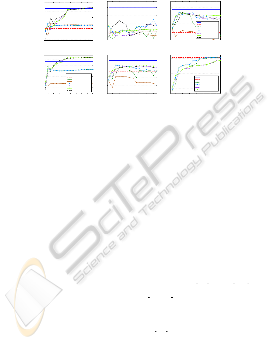
The left panel of Fig. 1 depicts the performance of the
LDA on the Pavia target image. Fig. 1(a) reports the
results obtained on the raw images, whereas Fig. 1(b)
shows the behavior after HM. One can notice the large
gap between in-domain (LDAtgt: solid blue line) and
out-domain (LDAsrc: dashed red line) models exist-
ing in both plots. Nonetheless, the impact of the HM
as a preprocessing step is quite remarkable. In fact,
LDA models trained on original target data outper-
form LDA models based on original source data by
0.356 κ points when no matching is performed, while
this difference reduces to 0.188 κ points after match-
ing.
In between these reference lines, we observe
two distinct trends. The first one concerns kernel-
based FE methods (LDA
KPCA: dashed purple line,
LDA KPCA 1DOM: solid light green line, LDA TCA:
dashed black line) that yield a robust performance
with accuracies reaching and even exceeding those of
ICPRAM2013-InternationalConferenceonPatternRecognitionApplicationsandMethods
422
2 4 6 8 10 12 14 16 18
0.2
0.3
0.4
0.5
0.6
0.7
0.8
Nr. of features
κ
2 4 6 8 10 12 14
0
0.2
0.4
0.6
0.8
Nr. of features
κ
2 4 6 8 10 12 14
0
0.2
0.4
0.6
0.8
Nr. of features
κ
QDAtgt
QDAsrc
QDA_PCA
QDA_PCA_INDEP
QDA_PCA_1DOM
QDA_KPCA
QDA_KPCA_1DOM
QDA_TCA
(a) (c) (e)
2 4 6 8 10 12 14 16 18
0.2
0.3
0.4
0.5
0.6
0.7
0.8
Nr. of features
κ
LDAtgt
LDAsrc
LDA_PCA
LDA_PCA_INDEP
LDA_PCA_1DOM
LDA_KPCA
LDA_KPCA_1DOM
LDA_TCA
2 4 6 8 10 12 14
0
0.2
0.4
0.6
0.8
Nr. of features
κ
2 4 6 8 10 12 14
0.5
0.6
0.7
0.8
0.9
Nr. of features
κ
LDAtgt
LDAsrc
LDA_PCA
LDA_PCA_1DOM
LDA_KPCA
LDA_KPCA_1DOM
(b) (d) (f)
Figure 1: Classification performances (average of estimated κ statistic over 10 runs) on the (left) Pavia and (right) Zurich
datasets considering several different settings. Target domain test sets included 14’047 (Pavia) and 26’797 (Zurich) samples.
(a) LDA on the Pavia target image, without HM. (b) LDA on the Pavia target image, with HM. (c) LDA on the Zurich target
image, without HM. (d) LDA on the Zurich target image, with HM. (e) QDA on the Zurich target image, with HM. (f) LDA
on the Zurich source image after FE, with HM (test set of 12’310 pixels). Legend of (b) also valid for (a), (c) and (d).
the target models when using at least 14 (no HM) or
8 (with HM) extracted features. After these thresh-
olds, the 3 techniques converge to very similar perfor-
mances, indicating the non-inferiority of KPCA with
respect to a domain adaptation technique as TCA.
Such a behavior also suggests that basing the FE on
one domain only (the source image) does not imply
a loss in invariance across domains. Indeed, rather
than the reduction of the statistical divergence be-
tween datasets (as measured by the MMD), it seems
that the extraction of features provides larger benefits
in terms of class discrimination. The latter is highly
increased in the two domains, especially when resort-
ing to kernel-based methods, easing thus the drawing
of meaningful and domain invariant class boundaries.
Note that the feature extractors employed in our tests
do not explicitly aim at optimizing class separation:
this may be interpreted as an implicit benefit of the
non-linear mapping.
The second trend is related to PCA-based meth-
ods (LDA PCA: dashed dark green line, LDA PCA 1DOM:
dashed light blue line), which reveal a less satisfactory
performance, just above the baseline of the LDAsrc
model. Peak accuracies are obtained in both exper-
iments with 2 features, while after, as noisy compo-
nents come into play, the quality of the LDA model
decreases. Also in this case, no difference is notice-
able between the use of both domains for FE versus
the use of the source domain only.
4.2 Zurich QuickBird Dataset
When considering the second dataset, Figs. 1(c) -(d)
confirm the usefulness of HM. All the meth-
ods/settings tested failed if applied to unmatched data.
Another key finding is the complementarity of the two
pre-classification procedures. On both datasets, we
noticed that the best accuracies are those reached by
models built on images with matched histograms hav-
ing undergone the FE. After these steps, the images
are sufficiently aligned and the features are discrimi-
nant enough to allow classifiers trained on the source
image to generalize well on the target image too.
Looking in details at Fig. 1(d), we witness a sim-
ilar behavior as with the Pavia dataset. Kernel-based
techniques need more features to attain good perfor-
mances with respect to PCA. On this dataset, nev-
ertheless, the best classification accuracy reached by
both families of methods is comparable and still 0.1
κ points below the reference of the target domain
model. Additionally, let us remark the slight superior-
ity of the setting in which the FE is done exclusively
on the source image (LDA PCA 1DOM, LDA KPCA 1DOM)
with respect to an extraction based on both domains
(LDA PCA, LDA KPCA). This trend, which is observable
also on the previously examined dataset, was not ex-
pected, revealing some interesting properties of the
tested approaches. Finally, as for the Pavia image,
we observe the complete, though expected, failure of
the LDA PCA INDEP approach (solid brown line), with
an accuracy curve evolving far below the rest of the
curves throughout the entire feature set.
Fig. 1(e) describes the behavior of the same align-
ment strategies, after HM, but when a non-linear clas-
sifier is used. The QDA curves depicted here show
that the tendencies highlighted for linear models are
InvestigatingFeatureExtractionforDomainAdaptationinRemoteSensingImageClassification
423

valid in this situation as well. It is worth noting the re-
markable discriminant and invariant properties of the
all the features extracted by KPCA from the source
image. The QDA KPCA 1DOM curve is the most sta-
ble across the entire range of features provided to the
model.
In conclusion, Fig. 1(f) uncovers the behavior of
some of the LDA models when asked, after HM and
after the projection, to predict the class labels back
on the source image. Although the pattern is not as
evident as expected, we can appreciate the loss in
accuracy induced by the FE based also on pixels is-
sued from another domain. This confirms that out-
domain data interfere with the proper extraction of
discriminant domain-specific features, while improv-
ing the overall generalization abilities of the system
when dealing with cross-domain knowledge transfer.
5 CONCLUSIONS
In this paper, the analysis of feature extraction tech-
niques to jointly transform two related remote sens-
ing images to align their feature spaces has been pre-
sented. After the projection, the matched images
display an increased discrimination between ground
cover classes, allowing a supervised classifier to ob-
tain an accurate generalization on both source and tar-
get domains.
Experiments proved that the combination of the
histogram matching procedure with the feature ex-
traction step is extremely beneficial, confirming the
mandatory application of the former before any do-
main adaptation task. Among the extraction tech-
niques, we noticed the slight superiority of kernel-
based features extractors (KPCA and TCA) with re-
spect to simple linear techniques such as PCA. No no-
table differences have been observed between the two
kernel methods. This fact suggests that, rather than
the reduction of the divergence between marginal dis-
tributions governing the two images, as pursued by
TCA, the key benefit is the increased class separabil-
ity. Also, we found that the use of pixels from one im-
age only to compute the projection provides equally
invariant features as a joint sampling of the images.
These results open a number of opportunities to
practitioners of the field dealing with large scale
land cover mapping applications involving several re-
motely sensed images.
As an outlook on new research directions, we plan
to test supervised FE methods. Techniques such as
Kernel Fisher Discriminant Analysis, Kernel Canon-
ical Correlation Analysis, Kernel Orthogonal Partial
Least Squares, etc. could be used to find the proper
projections based on the labeled source domain data.
ACKNOWLEDGEMENTS
This work has been supported by the Swiss National
Science Foundation with grants no. 200021-126505
and PZ00P2-136827.
REFERENCES
Arenas-Garc
´
ıa, J. and Petersen, K. B. (2009). Kernel mul-
tivariate analysis in remote sensing feature extraction.
In Camps-Valls, G. and Bruzzone, L., editors, Kernel
Methods for Remote Sensing Data Analysis. J. Wiley
& Sons, NJ, USA.
Borgwardt, K. M., Gretton, A., Rasch, M. J., Kriegel, H.-P.,
Sch
¨
olkopf, B., and Smola, A. J. (2006). Integrating
structured biological data by Kernel Maximum Mean
Discrepancy. Bioinformatics, 22(14):e49–e57.
Bruzzone, L. and Persello, C. (2009). A novel approach
to the selection of spatially invariant features for the
classification of hyperspectral images with improved
generalization capability. IEEE Trans. Geosci. Remote
Sens., 47(9):3180–3191.
Bruzzone, L. and Prieto, D. F. (2001). Unsupervised retrain-
ing of a maximum likelihood classifier for the analysis
of multitemporal remote sensing images. IEEE Trans.
Geosci. Remote Sens., 39(2):456–460.
Inamdar, S., Bovolo, F., and Bruzzone, L. (2008). Multidi-
mensional probability density function matching for
preprocessing of multitemporal remote sensing im-
ages. IEEE Trans. Geosci. Remote Sens., 46(4):1243–
1252.
Nielsen, A. A., Conradsen, K., and Simpson, J. J. (1998).
Multivariate alteration detection (MAD) and MAF
postprocessing in multispectral, bitemporal image
data: New approaches to change detection studies. Re-
mote Sens. Environ., 64:1–19.
Pan, S. J., Tsang, I., Kwok, J. T., and Yang, Q. (2011).
Domain adaptation via transfer component analysis.
IEEE Trans. Neural Netw., 22(2):199–210.
Pan, S. J. and Yang, Q. (2010). A survey on transfer learn-
ing. IEEE Trans. Knowl. Data Eng., 22(10):1345–
1359.
Sch
¨
olkopf, B., Smola, A., and M
¨
uller, K.-R. (1998). Non-
linear component analysis as a kernel eigenvalue prob-
lem. Neural Comput., 10(5):1299–1319.
Tuia, D., Mu
˜
noz-Mar
´
ı, J., Gomez-Chova, L., and Malo, J.
(2012). Graph matching for adaptation in remote sens-
ing. IEEE Trans. Geosci. Remote Sens., PP(99):1–13.
Woodcock, C. E., Macomber, S. A., Pax-Lenney, M., and
Cohen, W. B. (2001). Monitoring large areas for forest
change using Landsat: Generalization across space,
time and Landsat sensors. Remote Sens. Environ.,
78(1-2):194–203.
ICPRAM2013-InternationalConferenceonPatternRecognitionApplicationsandMethods
424
