
Visual Estimation of Object Density Distribution through Observation of
its Impulse Response
Artashes Mkhitaryan and Darius Burschka
Lab of Machine Vision and Perception, Technical University of Munich, Parkring 13, Garching bei Munich, Germany
Keywords:
Active Exploration, Object Categorization, Motion Analysis.
Abstract:
In this paper we introduce a novel vision based approach for estimating physical properties of an object such
as its center of mass and mass distribution. Passive observation only allows to approximate the center of mass
with the centroid of the object. This special case is only true for objects that consist of one material and
have unified mass distribution. We introduce an active interaction technique with the object derived from the
analogon to system identification with impulse functions. We treat the object as a black box and estimate its
internal structure by analyzing the response of the object to external impulses. The impulses are realized by
striking the object at points computed based on its external geometry. We determine the center of mass from
the profile of the observed angular motion of the object that is captured by a high frame-rate camera. We use
the motion profiles from multiple strikes to compute the mass distribution. Knowledge of these properties
of the object leads to more energy efficient and stable object manipulation. As we show in our real world
experiments, our approach is able to estimate the intrinsic layered density structure of an object.
1 INTRODUCTION
Major tasks in robotics such as object manipulation,
grasping, etc. often require physical interaction be-
tween robots and various objects. The success of
these interactions highly depends on the knowledge
about the physical properties of the manipulated ob-
ject such as roughness and stiffness of the surface, its
mass, and mass distribution.
Stiffness of the object is used to define suitable
power of grasp that will not break the object while
ensuring a stable grasp. The mass together with the
roughness of the surface of the object are used to pre-
vent slipping. Knowledge of the center of mass helps
to prevent undesired torques. Grasping away from the
center of mass can result in rotation of the object and
its eventual dropping. Mass distribution is used to es-
timate the interior state of the object which cannot be
observed otherwise.
To our knowledge, the current state of the art
methods for vision based graspless active estimation
of physical object properties do not address the issue
of estimating the mass distribution of the object, and
they either approximate the center of mass by the cen-
troid of the object or do not address it at all. We dis-
cuss this in more detail in Section 2. The goal of this
paper is to provide a way to estimate more detailed
Figure 1: Rotational motion.
physical information about the object which becomes
the more important the closer we operate to the ma-
nipulation limits of the mechanical gripper.
Miller and Allen introduce an approach for grasp
quality computation (Miller and Allen, 1999) where
they make an assumption that the center of mass is
located in the centroid of the object. This is mainly
true for objects that consist of single material with
unified mass distribution. However, this does not ap-
ply for most of the objects. Particularly for heavy
objects, the assumption can cause undesired torques
which will result in an unstable grasp. In (Kragic
et al., 2001), an online grasp planning approach is
described, where the authors require the information
about the mass and the center of mass of the object as
an input. Kunze et al. (Kunze et al., 2011) describe
a method for simulation based object manipulation.
They discuss in detail a case of robot manipulating an
egg. For this, they require information about physical
586
Mkhitaryan A. and Burschka D..
Visual Estimation of Object Density Distribution through Observation of its Impulse Response.
DOI: 10.5220/0004199705860595
In Proceedings of the International Conference on Computer Vision Theory and Applications (VISAPP-2013), pages 586-595
ISBN: 978-989-8565-47-1
Copyright
c
2013 SCITEPRESS (Science and Technology Publications, Lda.)

properties of the egg, i.e. the mass and stiffness of the
shell, the mass of the egg yolk, etc.
Since passive observation of an object is not suf-
ficient for estimation of its physical properties, an ac-
tive interaction is required. We adapt the analogy of a
widely used ’Black Box’ technique in system identi-
fication. We give an initial impulse to the object and
estimate its internal parameters from the resulting re-
sponse based on its external geometry and total mass.
In this paper, we present a vision based grasp-
less approach for estimating the center of mass and
the mass distribution. We use a bottom-up technique,
where we make an initial assumption about the cen-
ter of mass based on the external 3D geometry of the
object. This is used to compute possible points of in-
teraction between the robot and the object. We cor-
rect the center of mass by analyzing the observed ro-
tational motion (Fig. 1) resulting from the interaction,
and use it together with knowledge of total mass and
the external 3D geometry of the object to estimate the
mass distribution (Fig.2).
2 RELATED WORK
Most of the approaches for estimation of physical
properties of the objects require some direct interac-
tion between the robot and the object. These interac-
tions can be of various types, such as poking, striking,
tilting, grasping, etc. We break down the information
resulting from these interactions into three categories:
acoustic, visual (spatial/angular motion), and tactile.
In (Frank et al., 2010) a method for robot navi-
gation in an environment with deformable objects is
introduced, where the robot estimates the stiffness of
the object based on the tactile and visual information
acquired from poking. Femmam et al. (Femmam
et al., 2001) and Krotkov et al (Krotkov et al., 1995)
present an approach for characterizing the material of
the object based on its internal friction. Here they use
the acoustic information acquired from striking the
object. However, since the material type defines only
its molecular properties for the purpose of manipu-
lation this information is not sufficient. In (Krotkov,
1995) authors use both the visual and acoustic infor-
mation from strike to first estimate the mass of the ma-
terial then the type. Nevertheless the questions con-
cerning the mass distribution, and the center of mass
remain unresolved. Tanaka et al. (T.Tanaka et al.,
2003) introduce a method for constructing a reality
based virtual simulator. They use as input parameters
the mass and elasticity of the object, which are ex-
tracted from visual and tactile information acquired
by pushing. Here as well the extracted information
remains insufficient for purposes of object manipula-
tion. Yu et al. (Yu et al., 1999) present an approach
for estimating the mass and center of mass of the ob-
ject with previously unknown shape. For this, the au-
thors use tactile information acquired from tilting the
object from several points. However, the position of
the tilting points, and the stability of the tilts are not
addressed.
Our method uses the visual information acquired
while striking the object to estimate the center of
mass, the mass distribution, and the moment of inertia
of the object based on the given mass and the external
3D structure of the object. Thus it fills the gap in the
information required for object manipulation.
In Section 3, we describe our approach for esti-
mating the physical properties of the object. This sec-
tion is divided into three logical subsections:
• 3D model analysis (Sec. 3.1), where we com-
pute the robot/object interaction points based on
the appearance of the object.
• Estimation of the center of mass (Sec. 3.2), where
the center of mass is computed based on the pro-
file of the observed angular motion of the object.
• Estimation of mass distribution (Sec. 3.3), where
the mass distribution is computed based on the
profile of angular motion of the object and the
center of mass.
In Section 4, we describe the conducted experi-
ments, the experimental setup (Sec. 4.1), provide an
error sensitivity analysis of the approach (Sec. 4.2)
and present the results (Sec. 4.3, 4.4). We conclude
in section 5.
3 APPROACH
Our approach allows us to estimate physical proper-
ties, such as center of mass (CoM), moment of inertia
(MoI), and mass distribution of objects with unknown
internal structure. We require the mass m which could
be acquired by means described in (T.Tanaka et al.,
2003), (Krotkov, 1995) and the 3D model of the ex-
terior of the object, i.e the point cloud P = {p
i
} that
represents the surface of the mentioned object. This
can be acquired by laser scanner, stereo reconstruc-
tion, etc., as an input (Fig 2). By analyzing the 3D
point cloud (Sec. 3.1.1), we define possible points of
rotation (Sec. 3.1.2) around which we desire the ob-
ject to be rotated (Fig. 1). Later, we compute the cor-
responding interaction points (Sec. 3.1.3) that are the
places where the object should be struck by a robot to
achieve the desired rotation. The latter is defined as
VisualEstimationofObjectDensityDistributionthroughObservationofitsImpulseResponse
587

3D Model,
Mass
Center of
Mass
Mass
Distribution
Robot/Object
Interaction
Moment of
Inertia
Motion
Analysis
Search of
Coequal Mass
Regions
F
r
T
h
2
mg
Equi-Plane
R
1
R
3
R
2
A
B
C
Figure 2: State flow chart of the algorithm. (A) Illustrates
the robot/object interaction, here the top red dot is the im-
pact point and the bottom one is the rotation point. (B) Il-
lustrates the pose of the object when the gravity vector g
lies on the Equi-Plane. (C) Illustrates the search of three
coequal mass regions.
the rotation that is applied to the object for its transi-
tion from one stable pose to another. Typically these
rotations are around 90
◦
. We also estimate the ap-
proximate force by which the object should be struck.
After the strikes are performed, we analyze the profile
of the angular motion in time combined with the an-
gular acceleration profile to compute the initial MoI
along the axis of rotation (Sec. 3.3). As a final step
we use the CoM and the MoI along the axis of rotation
to compute the internal and external mass distribution
of the object, and to correct the estimate for MoI (Sec.
3.3.2).
3.1 3D Model Analysis
3.1.1 Initial Hypothesis for CoM
Given the point cloud P = {p
i
} and the mass m, we
make an assumption that the object consists of single
material, and that the mass distribution is almost uni-
form. This yields that the CoM should be located in
close proximity of the center p of the point cloud P.
That is, the CoM is located within the bounds of a re-
gion Q = {p
r
i
} that has its center at p. The former is
computed by means of a naive approach, where the
Principal Component Analysis (PCA) is performed
on the P having
p as the origin. The resulting eigen-
vectors ν
i
are treated as the axis of symmetry. We
define Q (Fig 3(a)) as a cuboid with center at p and
edges a
i
k ν
i
and ka
i
k = 2δ
i
where:
δ
i
= |
∑
(v
j
·ν
i
)<0
k v
j
k −
∑
(v
k
·ν
i
)>0
k v
k
k| + 1 (1)
v
i
= p
i
− p
Here v
i
are vectors that start at center point p and
end at p
i
∈ P and ν
i
are the above mentioned eigen-
vectors.
3.1.2 Extraction of Stable Equilibrium Planes,
and Rotation Points
Stable equilibrium planes are defined as planes on
which the object rests in a stable position, i.e. if the
object is tilted by a small degree in any direction the
resulting forces tend to bring it back to this resting po-
sition. To extract the stable equilibrium planes of the
object, we consider the set of points B ⊂ P that are lo-
cated on the convex hull of P. We fit planes {S
i
} ⊂ B
into the point cloud. In the next step, every set S
i
is
checked for stability. This is done by projecting Q on
to the plane represented by S
i
and checking if the pro-
jection of Q (CoM) lies completely within the convex
hull of the set of points S
i
, all the sets where this does
not hold are discarded as not stable resting positions.
In the following, we find all the planes S
i
that are par-
allel to each other, and discard the smaller ones. We
require that every object has at least two valid S
i
sets.
In case this does not hold, center of mass can be com-
puted by (Domokos and Vrkonyi, ry 7). We look at
the two largest sets {S
i
}, and for each of them per-
form a PCA over all the points in the set with origin at
the center p
s
i
of the corresponding set S
i
. Further, we
project a ray from every p
s
i
in direction of the corre-
sponding eigenvectors ν
s
i
j
derived from PCA, and de-
fine the points of intersection between the mentioned
rays and the convex hull of the corresponding set S
i
as
rotation point p
r
i
j
(Fig 3(b)). The line l
i j
of the convex
hull that contains p
r
i
j
, is defined as the axis of rotation.
3.1.3 Extraction of Impact Points and Forces
We consider the impact point good if it has the largest
possible lever and does not cause any torques during
the impact other than the one that acts along the axis
of rotation. Hence, we project the points {p
k
} ⊂ B to
find a good impact point for every rotation point p
r
i
j
,
that have normals to convex hull in the direction of
n
i j
= (
p
s
i
− p
r
i
j
), onto a plane that passes through p
r
i
j
and has a normal in the direction of n
i j
×n
s
i
, where n
s
i
is the normal of the plane S
i
. Further we define impact
point p
I
i j
by finding the closest point from {p
k
} to
the projected point that is the farthest from p
r
i
j
. Next
we proceed with computation of the minimal impact
force for achieving the desired rotation. Assume that
VISAPP2013-InternationalConferenceonComputerVisionTheoryandApplications
588
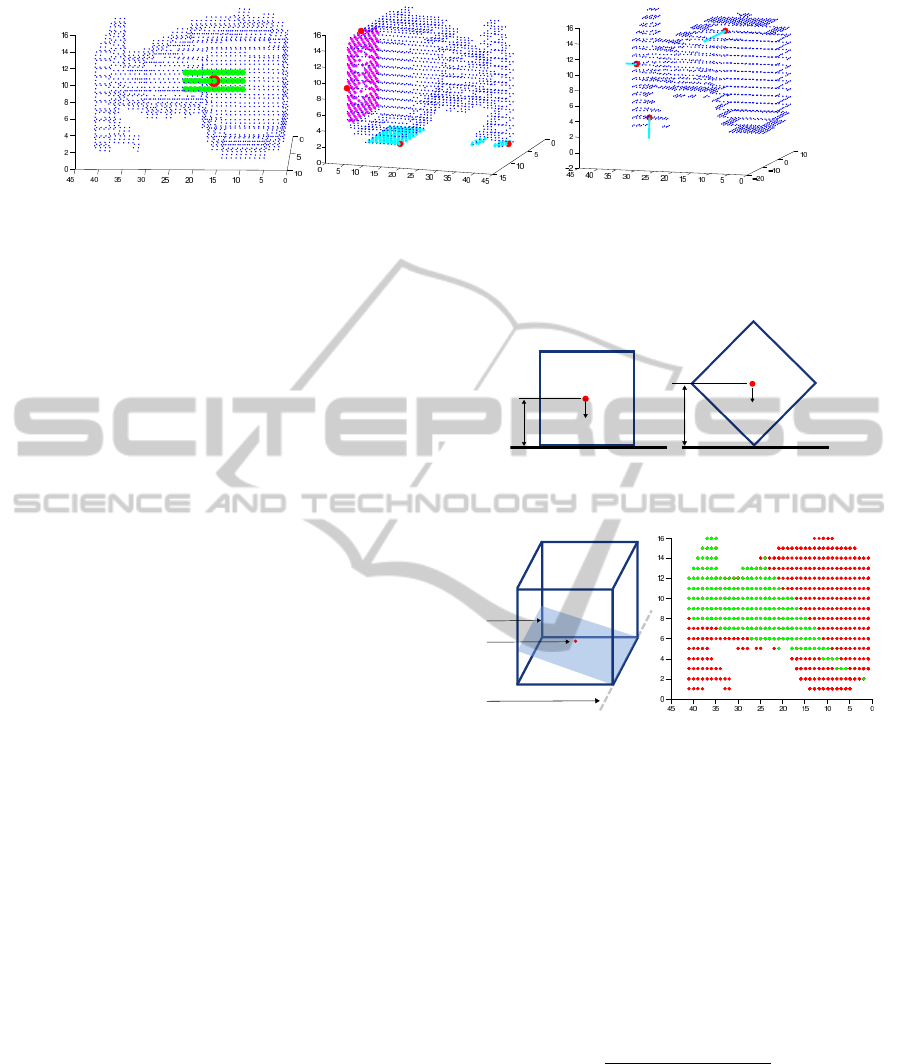
(a) Initial hypothesis for CoM (b) Stable Equilibrium Planes (c) Impact Forces
Figure 3: 3(a) Here the blue dots refer to point cloud P, the green dots to region Q, and the red dot to c. 3(b) Here the cyan and
magenta dots refer to stable planes {S
i
} and the red dots to rotation points p
r
i j
. 3(c) Here red dots refer to the impact points
p
I
i j
and the cyan lines to impact forces F
i j
.
the object initially has a potential energy mgh
1
, where
g is the acceleration caused by gravity, and h
1
is the
height of the CoM (Fig. 4(a)), the minimal amount of
energy required to achieve desirable rotation should
be equal to mg(h
2
− h
1
) + ε, where ε is an infinitely
small number, and h
2
is the distance between the CoM
and p
r
i
j
(Fig. 4(b)). The magnitude of the strike that
will cause the desired rotation for the point p
I
i j
can be
computed by:
Z
θ
1
+4θ
θ
1
F
i j
r
i j
sinθ dθ = mg(h
2
− h
1
) + ε (2)
where F
i j
is the impact force, r
i j
= p
I
i j
− p
r
i j
is the
displacement vector of force from the corresponding
rotation point, θ is the angle between F
i j
and r
i j
, 4θ
is the change of θ that occurs during the impact, and
the direction of the impact force is −n
i j
. Since at
this point the actual location of CoM is not known we
assume that for every impact point p
I
i j
the CoM is
located at that same impact point, and compute h
1
and
h
2
based on that assumption. Further, impact points
p
I
i j
with their corresponding forces F
i j
are sorted in
increasing fashion based on the magnitude of F
i j
, and
only the first 3 points are considered (Fig 3(c)).
3.2 CoM Estimation
In order to determine the position of center of
mass, only visual information about the object is not
enough. The robot should interact with the object.
This is realized by striking the object at the points p
I
i j
with the corresponding forces F
i j
. The information of
the resulting rotations is then used to extract the ap-
proximate positions of equi-planes. The latter is de-
fined as the plane which contains the center of mass
and the axis of rotation l
i j
(Fig. 5(a)). Further, the
Center of Mass is computed as a point of intersection
of 3 equi-planes.
h
1
mg
(a) before strike
h
2
mg
(b) entering stage two
Figure 4
.
Equi-Plane
CoM
Axis of Rotation
(a) (b)
Figure 5: In 5(a) Here the red dot is the CoM and the blue
plane is the Equi-plane. In 5(b) the figure shows the pro-
jection of P on to the plane P(p
r
i j
, l
i j
), where the green dots
∈ R
E
i j
.
3.2.1 Extraction of Equi-Planes
The basic physics behind the rotation, caused by a
strike is as follows. During the strike there are two
forces acting on the object, the striking force F
i j
by
robot and the gravity force mg. Therefore, during the
impact the object has an angular acceleration :
α =
F
i j
× r
i j
+ mg × r
m
i j
I
(3)
where I is the moment of inertia and r
m
i j
is the dis-
placement vector of CoM from the rotation point p
r
i
j
.
Note that here the moment of inertia I is a scalar ,
since the rotation is along single axis l
i j
. As a re-
sult when the strike is over, the object has some ini-
tial angular velocity which according to (2) is enough
to achieve the desired rotation. After the impact, the
VisualEstimationofObjectDensityDistributionthroughObservationofitsImpulseResponse
589
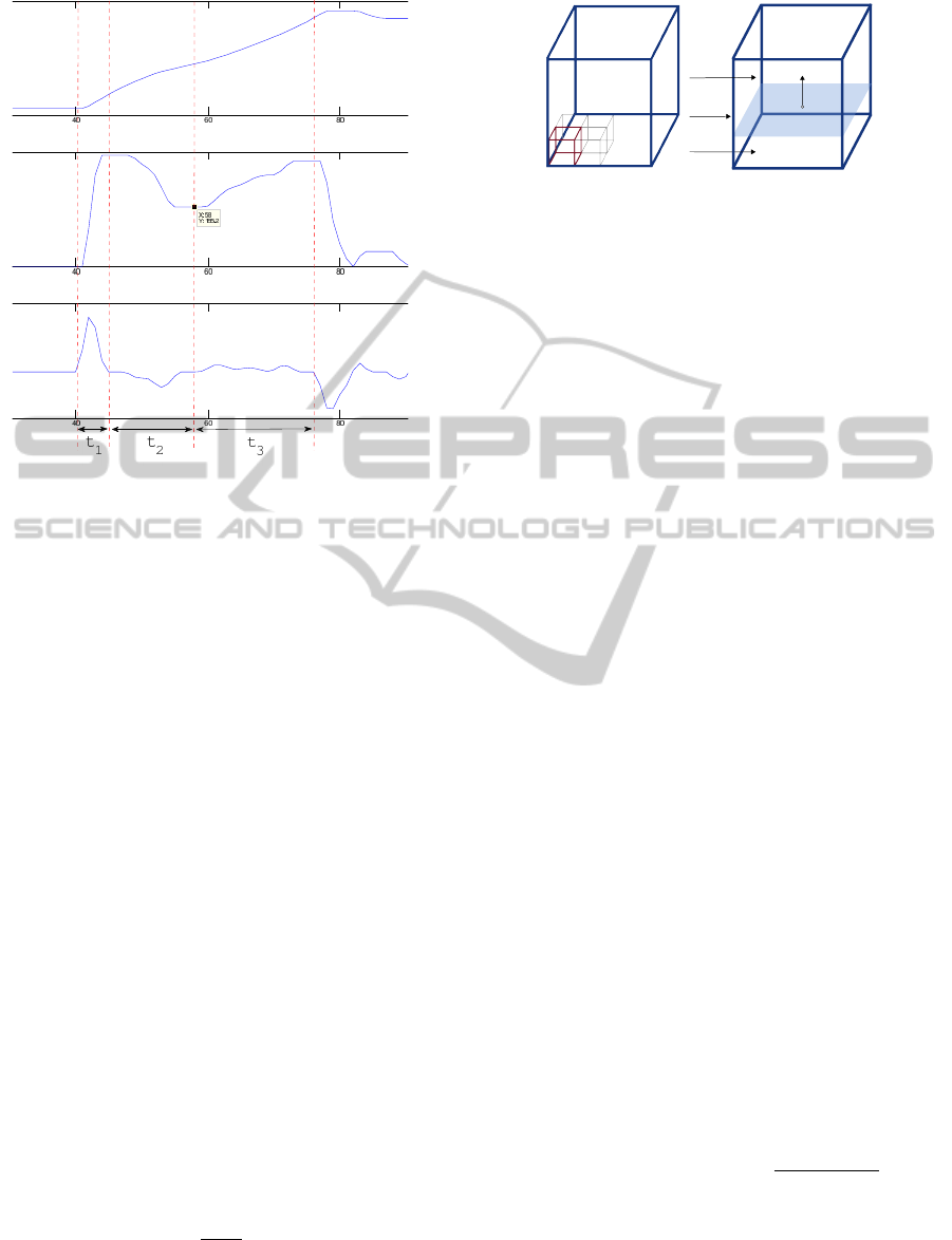
Figure 6: Here A) is the profile of angular motion, B) is
the profile of angular velocity and C) is the profile of ac-
celeration. t
1
is the duration of strike, t
2
is the duration of
stage one and t
3
is the duration of stage two. In all three
figures x = 58 is the point when the gravity vector lies in
the equi-plane.
object is influenced only by the gravity. This period
can be described in two stages (Fig. 6). In the first
stage the gravity force is trying to bring the object to
its initial position, i.e. the vector of angular accelera-
tion and the vector of angular velocity have opposite
directions. This is true until the point when the grav-
ity vector g lies entirely on the equi-plane. After, the
second stage begins. Here the gravity force is rotating
the object away from it’s initial pose, i.e. the vectors
of angular acceleration and angular velocity have the
same direction. Given as an input the angular pro-
file ang(t) of the rotation of the object over time, and
the angular acceleration profile acc(t) over time, we
extract the points (t
1
,t
2
, . . . ) in time when the angular
acceleration changes signs. Since the first sign change
is caused by ending of the strike, and the object enter-
ing stage one we discard t
1
. However, the second sign
change is a result of object ending stage one and en-
tering stage two. Thus we consider that at point t
2
the
angle between the equi-plane and the gravity vector is
quite small. In ideal case the gravity vector lies on the
equi-plane and thus the equi-plane E
i j
can be com-
pletely defined by the rotation point p
r
i j
and a normal
vector n
e
i j
, which can be computed by:
n
e
i j
= R
−g
k g k
× l
i j
(4)
where R is a rotation matrix that applies rotation by
the angle ang(t
2
) counter to the direction of angu-
(a)
R
1
R
3
R
2
(b)
Figure 7: In 7(a) illustration of the discretization of the ob-
ject by small cuboids. In 7(b) R
1
is the CRM bound to the
surface of the object, R
2
and R
3
are the CRMs bound to
lower and upper parts of the interior of the object corre-
spondingly.
lar velocity of the object, and l
i j
is a unit vector that
lies on the axes of rotation l
i j
. Note that in case of a
cylindrical object that has its center of mass lying on
its axes, the angular acceleration is constant at every
point in time, thus we can directly extract the equi-
plane.
3.2.2 Error Handling and Estimation of CoM
Ideally, the equi-planes can be defined by the rota-
tion point p
r
i
j
and a normal vector n
e
i j
. In this case
the center of mass would be located at the intersec-
tion point of three equi-planes, however this is never
the case. Since there are always errors that depend
on many parameters such as the actual angular ve-
locity, the sampling rate of the motion capturing de-
vice, and its internal errors. To cope with these errors,
we introduce a variable err that represents the errors
of the system. Instead of computing the equi-plane
E
i j
directly by means of (4), we define a region R
E
i j
that contains the true equi-plane (Fig. 5(b)). Here
R
E
i j
includes all the planes that pass through p
r
i j
and
have normals computed by (4) for the angles that lie
in [ang(t
2
) − err . . . ang(t
2
) + err]. Further we extract
the region of intersection of all the R
E
i j
-s and define
the center of mass as the centroid of that volume.
3.3 Estimation of Mass Distribution
Since in stage two (3.2.1) the object is effected only
by the gravity force, we consider MoI I
i j
for the rota-
tion axes that lie on l
i j
to be the average of all MoIs
computed for every point in time in stage two to:
I
i j
α = mkg × r
m
i j
k ⇒ I
i j
=
mkg × r
m
i j
k
α
(5)
On the other hand the MoI I
i j
can be computed
based on the mass distribution of the object. Assume
that the axes of rotation l
i j
are the z axes of Euclidean
space, then the MoI I
i j
would be I
zz
:
VISAPP2013-InternationalConferenceonComputerVisionTheoryandApplications
590

I
zz
=
ZZZ
V
(x
2
+ y
2
)ρdv (6)
Where ρ is the density of the object, dv is a differ-
ential volume element, x and y are the coordinates of
dv.
Further analysis of acquired data on rotational mo-
tion of the object allows us to compute a good esti-
mate of mass distribution of the object. The informa-
tion available at our disposal is the overall mass of the
object (1 parameter), the MoI for the rotation along
the particular axes (1 parameter), the CoM (2 param-
eters, since only orthogonal coordinates to rotation
axes contribute) and the external 3d structure of the
object (2 parameters). Thus for a particular rotation
the set of available parameters equals to 6. Since the
amount of parameters is limited the problem of esti-
mating the mass distribution can not be solved for the
most general case. However it is possible to compute
in some cases that will be described in the following
sections.
3.3.1 Discretization and Search of Mass
Distribution
The volume of the object is discretized by small cube
with d
3
dimensions. Every cuboid is considered to
consist of single material with mass m
i
and unified
mass distribution (Fig. 7(a)). Therefore the MoI dI
zz
at the CoM of every small cuboid can be computed
analytically to:
dI
zz
=
d
2
6
m
i
(7)
We define the regions in the object that have a
unified mass distribution as coequal mass regions
(CMR). For estimating the location and mass of each
region the number of parameters required is 3. These
are, the mass of the region (1 parameter ) and the loca-
tion (2 parameters). This means that in most general
case one can find a solution for the objects that con-
sist of two CMRs. However if one is not interested in
the exact shape and location of the CMRs in the ob-
ject and wants to get a general understanding of how
the masses are distributed in the object it is possible
to solve our problem for 3 CMRs. For 3 CMRs the
overall amount of parameters required is 9. However
if we bound one of the CMRs to the surface of the
object and define the border of the remaining two as
a plane (Fig. 7(b)) the amount of the required param-
eters will be 6. To find these masses and CMRs we
have to solve the discrete form of equation (6):
m
1
∑
R
1
(
d
2
6
+r
2
i
)+m
2
∑
R
2
(
d
2
6
+r
2
i
)+m
3
∑
R
3
(
d
2
6
+r
2
i
) = I
zz
(8)
where R
1
, R
2
, R
3
represent the three CMRs and r
i
=
p
x
2
+ y
2
is the displacement of the CoM of i-th cube
from the z axis. To solve (8) we use the parallel axes
theorem and compute the MoI for the rotation along
two other axes I
a
zz
, I
b
zz
and find the mass distribution by
solving the following equation:
a
1,1
a
1,2
a
1,3
a
2,1
a
2,2
a
2,3
a
3,1
a
3,2
a
3,3
m
1
m
2
m
3
=
I
zz
I
a
zz
I
b
zz
(9)
where a
i, j
are the corresponding coefficient of mass
m
j
from equation (8). To determine a
i, j
we perform
a sweep line search (Fig.7(b)) and solve the (9) for
every step of the search.
3.3.2 Extraction of Mass distribution, and
Correction of Moment of Inertia
As we already mentioned in 3.2.2 we believe that our
measurements are done within the bounds of certain
errors, thus we assume that the computed moment of
inertia I
i j
is not the true value. To cope with this prob-
lem, we expect that the true value of moment of in-
ertia lies withing the bonds of [I
i j
− dI
err
, I
i j
+ dI
err
]
region, where dI
err
is the estimated error of the mo-
tion capturing system. For every value of moment of
inertia within this scopes we perform the search for
the regions, and record all the valid results, i.e. the
results were all the estimated masses are positive and
m
1
+m
2
+m
3
= m holds. Next we compute the errors
of all the remaining estimations by computing the po-
sition of the CoM and comparing it to CoM position
from 3.2.2, considering the latter as ground truth. Fi-
nally we define the set {m
1
, m
2
, m
3
} with the small-
est error as the true solution, and its corresponding
MoI as the MoI along the considered axes. Since we
have three rotations along three different axes, in the
end our result is three sets of {m
1
, m
2
, m
3
}. We use
this to correct the estimation further by computing the
weighted average of all three masses. As weights, we
use the surface areas of the projected CMRs to the
plane that passes through the corresponding p
r
i j
rota-
tion point and has a normal l
i j
.
4 EXPERIMENTS AND RESULTS
4.1 Experimental Setup and
Experiments
In order to evaluate our approach the experiments
have been conducted on four different real world ob-
jects, square carton box, spray bottle, juice bottle and
VisualEstimationofObjectDensityDistributionthroughObservationofitsImpulseResponse
591

Figure 8: Objects.
a salt cylinder (Fig. 8). Each of these objects have
different masses and different mass distributions. As
a striker we used a metallic pendulum, since it gives
us the flexibility to repeat the experiments under the
same conditions multiple times, and its physics is well
known. We used a ‘Guppy Pro’ high frame rate cam-
era (120 fps) as a motion capture hardware, and a
square marker tracker for tracking the motion of the
object (Fig. 1). Each object was struck by pendulum
three times at each of the three different strike points.
In total 27 measurements were made. The algorithm
was implemented in Matlab and the computational
time depending on the volume of the object was from
30s up to 3 min. The point cloud was acquired by
‘David‘ laserscanner and was sampled down 3 times
to improve the computational time.
4.2 System Errors and Sensitivity of the
System to Errors
In this paper, we introduce a bottom up approach. We
start with an initial assumption about the center of
mass to define a robot/object interaction and correct
that assumption after the interaction was performed.
Further the center of mass is used to compute the mo-
ment of inertia for the particular axis of rotation, and
at the last step moment of inertia combined with cen-
ter of mass is used to compute the mass distribution of
the object. In this section we break down our system
into separate parts and discuss about the amount of er-
rors occurring in each of them and the error sensitivity
of each part.
To do this we use a carton box (Fig. 8) since
it is possible to compute the input values for every
stage analytically. Figure 9(a) illustrates the mea-
sured angle ang(t
2
) (section 3.2.1) for equi-plane de-
tection, that is extracted from the motion capture sys-
tem. Here the same object is rotated along the same
axis 27 times, the dashed blue line is the average
value over all the measurements. The standard devi-
ation over all measurements is 1.8484
◦
with around
4
◦
worst case scenario error. The measured angle
is further used to define the position of equi-planes
by (4). Further the center of mass is estimated from
equi-planes. Figure 9(b) demonstrates the relation of
the error for the estimated center of mass to the er-
ror of the measured angle ang(t
2
). Here one can see
that in case the measured error is 0 the resulting er-
ror in CoM is around 1.2mm. This is due to usage of
R
E
i j
(section 3.2.2) regions. It is possible to improve
this error by improving the quality of motion capture,
since the size of R
E
i j
region depends on it. Further we
estimate the moment of inertia by (5). Here the MoI
is linearly dependent on CoM and the angular accel-
eration α. Thus, the accumulated error should also be
of the same order. Finally, all this parameters are used
to estimate the mass distribution of the object. Figure
(9(c)) Illustrates the sensitivity of the estimate. Note
that in case the error of the estimated parameters is
zero then the estimated mass is precise. The gap in
the measured results is due to the fact that there are
no valid solutions for the particular input. However,
this issue is resolved in section 3.3.2 by using range
of possible MoIs. Here the dependency to the input
error is also linear. The sensitivity of the system to
the accuracy of the acquired point cloud is illustrated
in Fig. 10 . Here we introduce a random noise with
varying maximal magnitude (from .1-15 mm) to the
acquired point cloud, that was acquired by the ’David
laser scanner’. For each maximal noise magnitude we
measure the absolute distance between the estimated
CoM and the reference (Fig. 10(a)) as well as the
absolute weight difference between the estimated and
known three parts of the object (Fig. 10(b)).
4.3 Quantitative Assessment
The results of conducted experiments for center of
mass and mass distribution estimation are given in ta-
bles 1 and 2 correspondingly. Here, the reference val-
ues are given at the first row for every object, and the
estimated values are given on the following rows. For
the center of mass estimation (Table 1) the evaluation
of the results (column 6) is done by comparing the
volume V of the object and the volume V
s
(column 5),
where the latter is a sphere which has its center at the
reference point and the radius of the sphere is equal
to the distance d between the reference point and the
measured point (column 4). Here the average relative
error of our system is about 2% (Fig. 11(a)) and the
average absolute error is about 5.93mm. This results
are comparable to the ones introduced in (Yu et al.,
1999), where the average absolute error of the cen-
ter of mass estimation is around 2mm. However the
method for the center of mass estimation in (Yu et al.,
1999) is radically different from ours. There the CoM
is estimated from the tactile information acquired by
tilting the object, which has a mass of 1.872kg, where
VISAPP2013-InternationalConferenceonComputerVisionTheoryandApplications
592
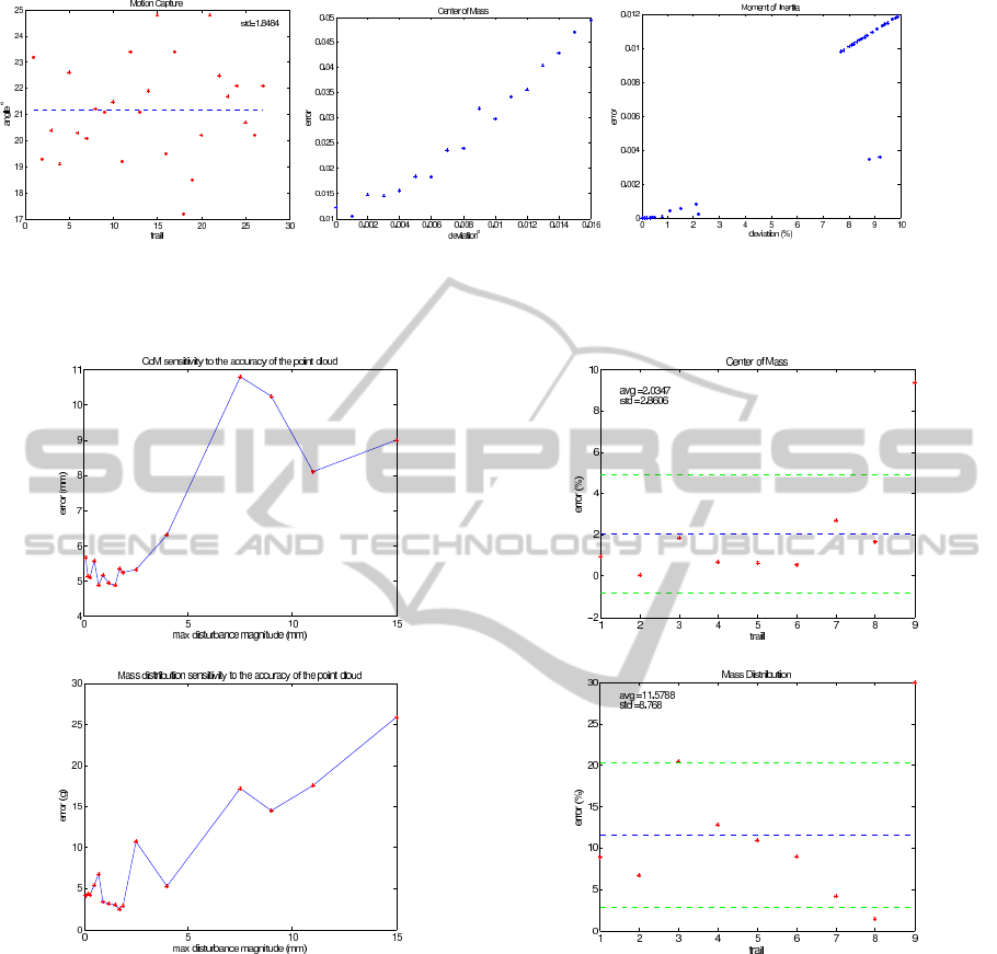
(a) Motion Capture System Error (b) CoM Sensitivity to Errors (c) MoI Sensitivity to Errors
Figure 9: Error Sensitivity of the System, here the units for measurements in 9(a) are degrees
◦
, for 9(b) the units are cm and
for 9(c) are kg ∗ m
2
.
(a) CoM sensitivity
(b) Mass distribution sensitivity
Figure 10: Sensitivity of mass distribution and center of
mass estimation to the accuracy of the point cloud.
the average weight of our objects is around 48g. Note
that the large mass results in dramatic improvement
in the estimation of the center of mass for both of the
approaches. Since in (Yu et al., 1999) the CoM is
computed from the force acquired by the force sen-
sors built in the robot arm, the signal to noise ration
depends on the mass of the object. As for our ap-
proach, we compute the CoM from the profile of an-
gular motion of the object, where the noise to signal
ratio is defined by the mass of the object and the ini-
tial impact force. The results for the mass distribution
estimation are presented in table 2. Since the masses
(a) Center of Mass
(b) Mass Distribution
Figure 11: Here the green dashed line represents the stan-
dard deviation and the blue dashed line is the average value.
of three CMRs of the object are not independent, the
measured errors for all three of them are also not in-
dependent. Thus, we define the error for a particular
object as the average error (column 4) over its CMRs.
Here we achieved the average relative error of 11.5%
11(b) and an average absolute error of 4.5g. The ob-
jects used for these experiments where the spray bot-
tle, juice bottle and the salt cylinder. The average size
of this objects is 6x20x5cm
3
, and the average weight
is 49g.
VisualEstimationofObjectDensityDistributionthroughObservationofitsImpulseResponse
593
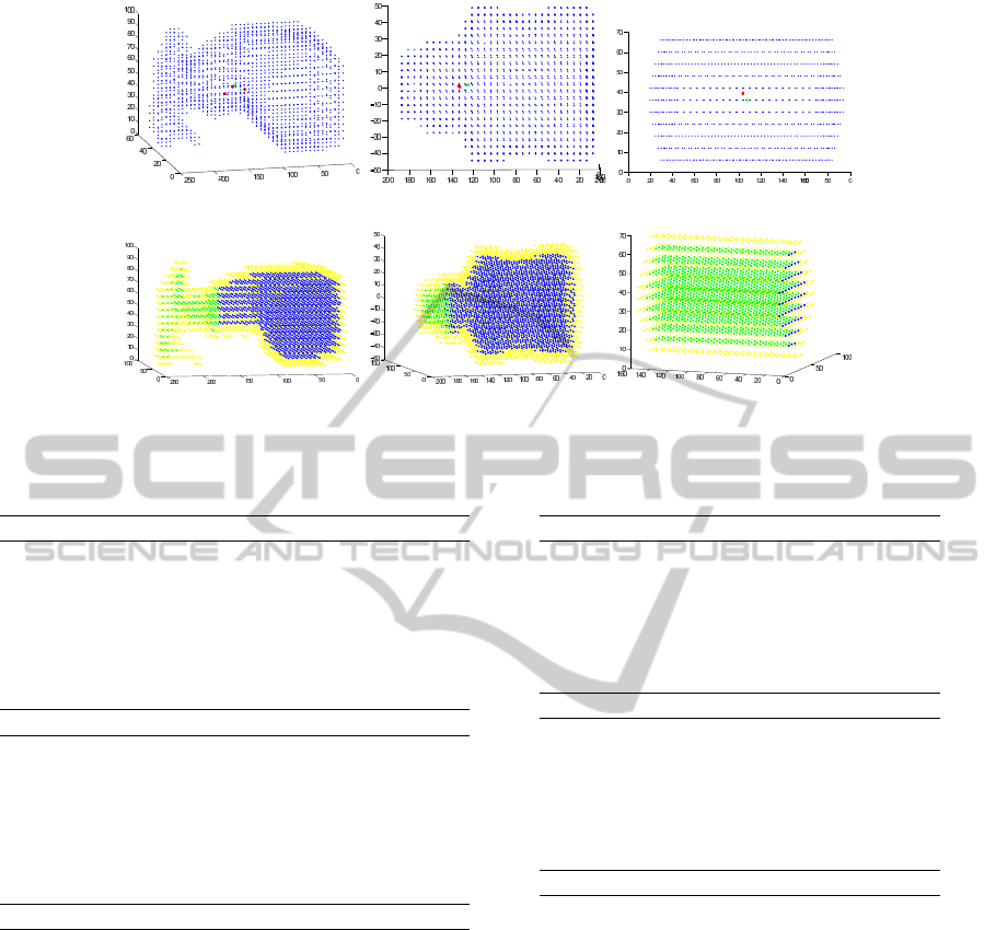
(a) Spray bottle CoM (b) Juice bottle CoM (c) Salt cylinder CoM
(d) Spray bottle mass distribution (e) Juice bottle mass distribution (f) Salt cylinder mass distribution
Figure 12: Experimental Results for Qualitative Assessment.
Table 1: Experimental Results, Center of Mass.
Spray bottle V = 812592mm
3
Ref. Res. 1 Res. 2 Res. 3
x(mm) 34.3387 30.3355 33.3702 33.9160
y(mm) 135.298 124.748 140.034 150.198
z(mm) 50.8100 49.4065 50.1787 44.5418
d(mm) 0.0 12.3410 3.91080 15.2545
V
s
(mm
3
) 0.0 7874 250 14869
err(%) 0 0.9691 0.0308 1.8298
Juice bottle V = 862704mm
3
Ref. Res. 1 Res. 2 Res. 3
x(mm) 68.9777 60.8626 62.1442 62.2436
y(mm) 123.717 131.418 132.627 131.961
z(mm) -0.5890 -2.0172 -1.2440 -1.4216
d(mm) 0.0 11.0720 10.899 10.313
V
s
(mm
3
) 0.0 5687 5424 4596
err(%) 0 0.6592 0.6287 0.5327
Juice bottle V = 862704mm
3
Ref. Res. 1 Res. 2 Res. 3
x(mm) 36.0000 51.0000 48.8571 53.1429
y(mm) 81.0000 84.0000 83.1489 84.8371
z(mm) 36.0000 39.0000 38.5714 39.4286
d(mm) 0.0 15.588 13.285 23.708
V
s
(mm
3
) 0.0 15867 9823 55818
err(%) 0 2.6596 1.6465 9.3562
4.4 Qualitative Assessment
For qualitative assessment the results from the exper-
iments are illustrated in Fig. 12. The first row of the
illustration demonstrates the results for the CoM es-
timation. Here the green dot represents the center of
mass of the object, and the red dotes are the estimated
position. The second row visualizes the result for es-
timation of mass distribution. For the spray bottle,
the region represented by yellow dots is estimated to
Table 2: Experimental Results, Mass Distribution.
Spray bottle, M = 57g
Ref Res. 1 Res. 2 Res. 3
surf.(g) 35.0 27.4 29.3 17.4
top(g) 22.0 25.6 22.6 29.3
bot.(g) 0.00 4.10 5.10 10.0
err.(g) 0.00 5.06 3.80 11.6
err.(%) 0.00 8.88 6.66 20.4
Juice bottle, M=56g
Ref Res. 1 Res. 2 Res. 3
surf.(g) 30.0 36.0 30.1 29.8
top(g) 26.0 12.7 16.3 18.2
bot.(g) 0.00 6.00 8.50 7.00
err.(g) 0.00 7.16 6.10 5.00
err.(%) 0.00 12.7 10.8 8.92
Salt cylinder, M=34g
Ref Res. 1 Res. 2 Res. 3
surf.(g) 32.0 30.2 31.1 17.8
top(g) 2.00 3.80 2.30 10.6
bot.(g) 0.00 0.20 0.10 6.00
err.(g) 0.00 1.33 0.46 9.60
err.(%) 0.00 4.16 1.45 30.0
have weight of 29.3g, green dots 22.6, and blue dots
5.1. Note that here the bottle is empty and the only
thing that the blue region contains withing itself is the
tube for pumping out the liquid. For juice bottle, the
yellow region has an approximate wight of 29.8g, the
blue region representing the container part has weight
of 7g, and the green region that represents the cap has
a weight of 18.2g. Here the container is also empty.
For the empty salt cylinder, the estimated weights are
31g, 2.3g, 0.1g for the yellow, blue and green regions
correspondingly.
VISAPP2013-InternationalConferenceonComputerVisionTheoryandApplications
594
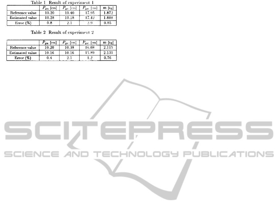
Figure 13: Experimental results for center of mass estima-
tion, by (Yu et al., 1999).
5 CONCLUSIONS
In this paper we described a real robotic system for es-
timating such physical properties of the object as its
center of mass and mass distribution. These parame-
ters are crucial for making object manipulation more
energy efficient and stable. Our approach allows the
robot to observe the physical properties of the object
that are visually unobservable. It has minimal hard-
ware requirements on the robot, i.e. it requires a sin-
gle high frame rate camera, and a robot hand. Initially,
our approach defines a stable interaction between the
robot and the object based on the visual appearance
of the object, and estimates the physical parameters
from the analysis of the profile of rotational motion.
As we have shown in Section 4.2, the error propaga-
tion from estimation of one parameter to another is
linear. We managed to achieve an average relative er-
ror of 2% for center of mass estimation, and of 11%
for mass distribution for real world objects, which to
outperforms most current state of the art methods.
ACKNOWLEDGEMENTS
This work was supported by the European Communi-
tys Seventh Framework Programme FP7/2007-2013
under grant agreement 215821 (GRASP project).
REFERENCES
Domokos, G. and Vrkonyi, P. L. (2008 January 7). Ge-
ometry and self-righting of turtles. Proc Biol Sci,
275(1630):11–17.
Femmam, S., MSirdi, N. K., and Ouahabi, A. (OCTOBER
2001). Perception and characterization of materials
using signal processing techniques. In IEEE Transac-
tions on Instrumentation and Measurement, Vol. 50,
No. 5.
Frank, B., Schmedding, R., Stachniss, C., Teschner, M., and
Burgard, W. (2010). Learning deformable object mod-
els for mobile robot navigation. In Science and Sys-
tems Conference (RSS).
Kragic, D., Miller, A. T., and Allen, P. K. (2001). Real-
time tracking meets online grasp planning. In IEEE
International Conference on Robotics & Automation.
Krotkov, E. (1995). Robotic perception of material. In Pro-
ceedings of the International Joint Conference Artifi-
cal Intelligence.
Krotkov, E., Klatzky, R., and Zumel, N. (1995). Robotic
perception of material: Experiments with shape-
invariant acoustic measures of material type. In
Preprints of the fourth international symposium on ex-
perimental robotics, iser (not sure).
Kunze, L., Dolha, M. E., Guzman, E., and Beetz, M.
(2011). Simulation-based temporal projection of ev-
eryday robot object manipulation. In Proc. of the 10th
Int. Conf. on Autonomous Agents and Multiagent Sys-
tems (AAMAS 2011).
Miller, A. T. and Allen, P. K. (1999). Examples of 3d grasp
quality computations. In IEEE International Confer-
ence on Robotics & Automation.
T.Tanaka, H., Kushihama, K., Ueda, N., and ichi Hirai, S.
(2003). A vision-based haptic exploration. In Inter-
national Conference on Robotics & Automation.
Yu, Y., Fukuda, K., and Tsujio, S. (1999). Estima-
tion of mass and center of mass of graspless and
shape-unknown object. In InternationalConference on
Robotics & Automation.
VisualEstimationofObjectDensityDistributionthroughObservationofitsImpulseResponse
595
