
Optical Flow Estimation with Consistent Spatio-temporal
Coherence Models
Javier S
´
anchez, Agust
´
ın Salgado and Nelson Monz
´
on
Centro de Tecnolog
´
ıas de la Imagen (CTIM), Departamento de Inform
´
atica y Sistemas,
University of Las Palmas de Gran Canaria, Las Palmas de Gran Canaria, Spain
Keywords:
Optical Flow, Variational Methods, PDE, Temporal Coherence.
Abstract:
In this work we propose a new variational model for the consistent estimation of motion fields. The aim of
this work is to develop appropriate spatio-temporal coherence models. In this sense, we propose two main
contributions: a nonlinear flow constancy assumption, similar in spirit to the nonlinear brightness constancy
assumption, which conveniently relates flow fields at different time instants; and a nonlinear temporal regular-
ization scheme, which complements the spatial regularization and can cope with piecewise continuous motion
fields. These contributions pose a congruent variational model since all the energy terms, except the spatial
regularization, are based on nonlinear warpings of the flow field. This model is more general than its spatial
counterpart, provides more accurate solutions and preserves the continuity of optical flows in time. In the
experimental results, we show that the method attains better results and, in particular, it considerably improves
the accuracy in the presence of large displacements.
1 INTRODUCTION
The estimation of motion fields is a key problem in
computer vision. It serves as a basis for many appli-
cations, such us stereoscopic vision and 3D scene re-
construction, medical image analysis, structure from
motion, object tracking and others. If we are given
a video sequence, and we want to find the motion of
the objects in the images, our method should provide
a solution that is consistent through the sequence. In
this work, we address the problem of temporal co-
herence in optical flow methods. The aim is to devise
new methods that allow finding continuous flow fields
in time.
Optical flow methods can be further improved if
temporal information is properly managed (Weickert
and Schn
¨
orr, 2001). In this work, the authors propose
a method that is a straight extrapolation of the spatial
coherence model to the temporal dimension, based on
a continuous spatio-temporal regularization scheme.
More recently, some authors have generalized the use
of the flow temporal derivative. Typically, the tem-
poral information is coupled with the spatial gradient
in the form of a non-quadratic 3D smoothing opera-
tor. However, in (S
´
anchez et al., 2012), the authors
analyze the behavior of a continuous temporal regu-
larizer and show several experiments where it fails.
Black (Black, 1994) uses robust functionals to
deal with outliers and introduces a temporal continu-
ity strategy to account for the temporal coherence of
the sequence. This temporal continuity is based on a
prediction step and an attachment of the flow to the
predicted value. It warps the flow field to estimate its
value in the following frame. This is interesting, be-
cause the warping allows finding the correct flow cor-
respondences. More recently, there has been several
works dealing with temporal coherence in different
ways: for instance, in (Sun et al., 2010) the temporal
consistency is established reasoning on the segmenta-
tion on layers.
We propose several contributions: on the one
hand, we introduce a nonlinear flow constancy as-
sumption that fits with the nonlinear data assump-
tion; on the other hand, we propose a novel non-
linear flow regularization scheme that can deal with
non-continuous optical flows. Another contribution
is a new anistropic diffusion operator based on the
Nagel-Enkelmann operator. This new operator allows
respecting the object boundaries during the diffusion
process, at the same time that it avoids oversegmenta-
tion in texture regions.
The former contribution was motivated by the re-
sults presented in (Salgado and S
´
anchez, 2006). The
experimental results showed that the use of a nonlin-
366
Sánchez J., Salgado A. and Monzón N..
Optical Flow Estimation with Consistent Spatio-temporal Coherence Models.
DOI: 10.5220/0004199903660369
In Proceedings of the International Conference on Computer Vision Theory and Applications (VISAPP-2013), pages 366-369
ISBN: 978-989-8565-48-8
Copyright
c
2013 SCITEPRESS (Science and Technology Publications, Lda.)

ear temporal formulation of the flow field provided
very good results. That was the first time that such
a nonlinear flow assumption was introduced. For the
second contribution, we introduce a non-continuous
flow regularization scheme at the PDE level. This is
a pure regularization approach that replaces the tradi-
tional continuous temporal smoothing.
In Section 2 we examine the new energy model
and explain the novel temporal coherence strategy.
The minimization of the energy model and some nu-
merical details are explained in Section 3. In the ex-
perimental results – Section 4 – we test our method
using a synthetic sequence. Finally the conclusions in
Section 5.
2 NONLINEAR VARIATIONAL
MODEL
If we have a set of images I
j
(x), with j = 1, .., N,
N the number of frames and x = (x, y), the aim is
to find a set of optical flow functions,
{
h
i
(x)
}
, with
i = 1, .., N −1. We decompose our energy functional
in two separate parts:
E (
{
h
i
(x)
}
) = E
S
(
{
h
i
(x)
}
) + E
T
(
{
h
i
(x)
}
). (1)
The first term on the right, E
S
, stands for the spa-
tial energy model and the second term, E
T
, is the en-
ergy model corresponding to the temporal coherence
strategy. The spatial model reads as follows:
E
S
=
Z
N−1
∑
i=1
Ψ
(I
i
(x) −I
i+1
(x + h
i
(x)))
2
dx
+ γ
Z
N−1
∑
i=1
Ψ
k
∇I
i
(x) −∇I
i+1
(x + h
i
(x))
k
2
dx
+ α
Z
N−1
∑
i=1
Ψ(N (∇I
i
, ∇h
i
))dx, (2)
with Ψ
s
2
=
√
s
2
+ ε
2
(ε a prefixed small con-
stant, e.g. 0.01). This kind of function mitigates
the effect of outliers and behaves like TV regu-
larization approaches when used in the smoothness
term. The advantage of a TV smoothing scheme
is that it preserves discontinuities of the flow. We
use the anisotropic diffusion operator, N (∇I
i
, ∇h
i
) =
trace
∇h
T
i
(x)D(∇I
i
)∇h
i
(x)
, proposed in (Nagel
and Enkelmann, 1986), which preserves discontinu-
ities of the images in the flow field, D(.) defined as:
D(∇I) =
∇I
⊥T
∇I
⊥
+ λ
2
Id
k
∇I
k
2
+ 2λ
2
,
with Id the identity matrix. λ determines the gradient
value from which the anisotropy is activated. This
parameter can be computed from the more intuitive
isotropic fraction, 0 ≤ s ≤ 1, introduced in (
´
Alvarez
et al., 2000).
For the temporal energy model, we follow the
ideas presented in (Salgado and S
´
anchez, 2006).
Given that an object in the sequence may undergo
large displacements, we have to deal with informa-
tion that is warped through the flows. In fact, given a
flow h
i
(x), at instant i, its corresponding flow in the
following time instant is h
i+1
(x + h
i
(x)). If h
i
(x) is
large, then the temporal derivative cannot be com-
puted, but the previous correspondence still holds.
Thus, one way to relate motion fields at different
time instants is through the flow constancy assump-
tion (FCA), h
i
(x) = h
i+1
(x + h
i
(x)). Therefore, the
temporal coherence model, E
T
, can be formulated as,
E
T
= β
Z
N−2
∑
i=1
Φ
k
h
i
(x) −h
i+1
(x + h
i
(x))
k
2
dx,
(3)
with Φ
s
2
= e
−k∇Ik
κ
√
s
2
+ ε
2
, with κ = 0.8 and ε =
0.01.
This term is congruent with the brightness and
gradient constancy terms. In the presence of large
displacements, this temporal model is coherent with
the spatial formulation and relates values at the cor-
rect positions. Note that when object displacements
are very small, this term can be seen as an approxi-
mation of the temporal derivative of the flow, which
has shown to be effective in a continuous setting (e.g.,
(Weickert and Schn
¨
orr, 2001) or (Papenberg et al.,
2006)).
3 MINIMIZING THE ENERGY
MODEL
In this section we derive the Euler-Lagrange equa-
tions of (2) and (3). Then, we introduce a nonlinear
regularization scheme at the PDE, which closely re-
sembles a continuous temporal smoothing approach.
The Euler-Lagrange equations for the spatial en-
ergy model (2) are:
0 =Ψ
0
(I
i
(x) −I
i+1
(x + h
i
(x)))
2
·(I
i
(x) −I
i+1
(x + h
i
(x))) ·∇I
i+1
(x + h
i
(x))
+ γ Ψ
0
k
∇I
i
(x) −∇I
i+1
(x + h
i
(x))
k
2
·(∇I
i
(x) −∇I
i+1
(x + h
i
(x))) ·H I
i+1
(x + h
i
(x))
+ α div
Ψ
0
(N (∇I
i
, ∇h
i
)) ·D(∇I
i
) ·∇h
i
, (4)
OpticalFlowEstimationwithConsistentSpatio-temporalCoherenceModels
367

where H I
i+1
is the Hessian matrix. The temporal en-
ergy model (3) yields the following Euler-Lagrange
equations:
0 =β Φ
0
k
h
i
(x) −h
i+1
(x + h
i
(x))
k
2
·
(h
i
(x) −h
i+1
(x + h
i
(x)))
T
·
Id −∇h
T
i+1
(x + h
i
(x))
+ β Φ
0
h
i
(x) −h
i−1
(x + h
∗
i−1
(x))
2
·
h
i
(x) −h
i−1
(x + h
∗
i−1
(x))
·
|
J (x)
|
, (5)
where
|
J (x)
|
stands for the absolute value of the Jaco-
bian matrix, with J (x) =
1 + u
∗
i−1,x
1 + v
∗
i−1,y
−
u
∗
i−1,y
v
∗
i−1,x
. h
∗
i−1
=
u
∗
i−1
, v
∗
i−1
T
is the backward flow
from frame I
i
to I
i−1
.
In order to derive (h
i
(x) −h
i+1
(x + h
i
(x))) with
respect to h
i+1
(x), we can use the change of variables
z = x + h
i−1
(x). This change allows us to remove the
nonlinearity inside the flow. The backward flow, h
∗
i−1
,
naturally appears due to this change of variables.
We use a gradient descent approach to find the so-
lution of the above PDE. The nonlinear terms, e.g.
I
i+1
(x + h
i
(x)), are linearized using first order Tay-
lor expansions. In the temporal coherent framework,
we use Dirichlet boundary conditions for the last and
first frames, whereas Neumann boundary conditions
are used in the spatial domain. We use a standard
coarse-to-fine strategy to deal with large displace-
ments, based on a pyramidal structure. The system
of equations is sparse, so it can be efficiently solved
by means of the Gauss-Seidel or SOR method in each
scale.
We introduce a nonlinear temporal smoothing
scheme. Its formulation is intuitively derived from
the second order temporal derivative of the flow field,
u
tt
≈ u
i, j,k+1
−2u
i, j,k
+ u
i, j,k−1
. In the PDE, this sec-
ond order derivative has a continuous temporal regu-
larizing effect that is consistent if the flow field varies
smoothly across the image sequence. We propose a
new solution, which is similar in spirit to this numer-
ical approximation, and is suitable for dealing with
non-continuous displacements. This is a nonlinear
formulation that puts into correspondence the correct
flow values in different frames. It is not evident how
to abstract this idea at the energy level in Equation
(3). As before, we also use L
1
functions to turn the
method more robust against outliers, in the following
way:
T
S
=δ Φ
0
h
i−1
(x + h
∗
i−1
(x)) −h
i+1
(x + h
i
(x))
2
·
h
i−1
(x + h
∗
i−1
(x)) −2h
i
(x) + h
i+1
(x + h
i
(x))
(6)
This term provides a new scheme at the PDE level
and has to be combined with the previous PDE equa-
tions (4) and (5). In the experiments, we show that
this nonlinear smoothing provides very good results:
it has a similar gain as in the continuous case, but it
correctly handles large discontinuities in the motion
field.
4 EXPERIMENTAL RESULTS
Next we examine the behavior of the temporal mod-
els introduced in equations (1) and (6). For this, we
use a simple sequence of a square translating over a
textured background. The square is moving 15 pixels
per frame, while the background moves 3 pixels in the
same direction. In the first row of Fig. 1, we show the
third frame of the square sequence, its ground truth,
and the best spatial solution found. In the second row,
we show three temporal solutions: the first for the
nonlinear temporal attachment defined in (3); the sec-
ond, for the nonlinear temporal smoothnes approach
defined in (6); and, finally, using both temporal terms.
The color, in the motion field, represents the direction
and, the intensity, its magnitude.
Figure 1: Square sequence. First row: one of the images of
the Square sequence, the ground truth and the best spatial
solution found. Second row: three temporal solutions with
β = 8, δ = 25 and (β = 1, δ = 25), respectively.
The improvement of the temporal methods with
respect to the spatial solution is important. As ex-
pected, the spatial method produces higher errors at
the motion discontinuities and, more significantly, at
the occlusions. Table 1 shows the average End-point
(EPE) and Angular (AAE) errors for these results.
The first temporal result, corresponding to the first im-
age in the second row of Fig. 1, provides an important
improvement on the EPE and, more noticeable, on the
AAE. The improvement in accuracy is still more im-
portant if we use the nonlinear temporal smoothing
scheme (Equation (6)) or a combination of both.
We observe that the nonlinear temporal smooth-
ing scheme (6) behaves better than the temporal at-
tachment, even at the motion boundaries. The graph-
ics in Fig. 2 show the EPE for every frame on the
VISAPP2013-InternationalConferenceonComputerVisionTheoryandApplications
368
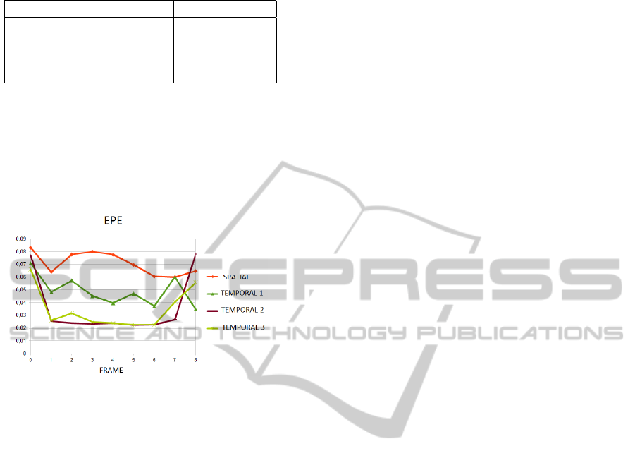
Table 1: EPE and AAE for the Square sequence.
Method EPE AAE
Spatial 0.071 0.629
o
Temporal 1 (β = 8) 0.049 0.204
o
Temporal 2 (δ = 25) 0.036 0.134
o
Temporal 3 (β = 1, δ = 25) 0.035 0.138
o
square sequence. Frame by frame, the optical flows
are more accurate in the temporal methods. We also
observe that the results are very stable, especially in
the middle of the ’Temporal 2 (δ)’ line. Reasonably,
the frames at the beginning and end of the sequence
present higher errors, due to the Dirichlet boundary
conditions.
Figure 2: EPE in each optical flow of the Square sequence.
5 CONCLUSIONS
In this paper we have presented a new spatio-temporal
coherence model for the consistent estimation of op-
tical flows. We have focused on different nonlinear
flow assumptions that are more confident in the es-
timation of motion fields than previous approaches.
These nonlinear assumptions correctly fit with the
standard nonlinear brightness and gradient constancy
terms, can cope with general image sequences and
provide better solutions. In particular, we have pro-
posed two main contributions: on the one hand, we
have introduced the nonlinear flow constancy assump-
tion (FCA) in the energy model. This term relates
flow fields at different time instants and is consis-
tent with the rest of the energy terms. On the other
hand, we have proposed a nonlinear temporal diffu-
sion scheme at the PDE level, which produces con-
tinuous flows in time. We have seen that this new
scheme is more general than using the continuous
temporal regularization of the flow, with the advan-
tage that it conveniently deals with continuous and
non-continuous velocities. In fact, if the motion is
very small, this term approximates a continuous tem-
poral smoothing scheme. In the experimental results,
we have shown that the method provides important
accuracy improvements, specially in the presence of
large displacements. The results are promising in both
cases, although we observe a better performance for
the nonlinear temporal smoothing scheme in general.
Another interesting result of the temporal coherence
schemes is that the background motion oscillations
tend to disapper. These oscillations clearly appear in
the spatial method, in regions where there is no appar-
ent motion.
ACKNOWLEDGEMENTS
This work has been partly founded by the Spanish
Ministry of Science and Innovation through the re-
search project TIN2011-25488.
REFERENCES
´
Alvarez, L., Weickert, J., and S
´
anchez, J. (2000). Reli-
able estimation of dense optical flow fields with large
displacements. International Journal of Computer Vi-
sion, 39(1):41–56.
Black, M. J. (1994). Recursive non-linear estimation of dis-
continuous flow fields. In Proceedings of the third Eu-
ropean conference on Computer vision (vol. 1), ECCV
’94, pages 138–145, Secaucus, NJ, USA. Springer-
Verlag New York, Inc.
Nagel, H. H. and Enkelmann, W. (1986). An investigation
of smoothness constraints for the estimation of dis-
placement vector fields from image sequences. IEEE
Transanctions on Pattern Analysis and Machine Intel-
ligence, 8:565–593.
Papenberg, N., Bruhn, A., Brox, T., Didas, S., and Weick-
ert, J. (2006). Highly Accurate Optic Flow Compu-
tation with Theoretically Justified Warping. Interna-
tional Journal of Computer Vision, 67(2):141–158.
Salgado, A. and S
´
anchez, J. (2006). A temporal regularizer
for large optical flow estimation. In IEEE Interna-
tional Conference on Image Processing ICIP, pages
1233–1236.
S
´
anchez, J., Monz
´
on, N., and Salgado, A. (2012). Robust
optical flow estimation. IPOL: Image Processing On-
line, Preprint:1–18.
Sun, D., Sudderth, E., and Black, M. J. (2010). Lay-
ered Image Motion with Explicit Occlusions, Tempo-
ral Consistency, and Depth Ordering. In Lafferty, J.,
Williams, C. K. I., Shawe-Taylor, J., Zemel, R., and
Culotta, A., editors, Advances in Neural Information
Processing Systems 23, volume 23, pages 2226–2234.
Weickert, J. and Schn
¨
orr, C. (2001). Variational Optic
Flow Computation with a Spatio-Temporal Smooth-
ness Constraint. Journal of Mathematical Imaging
and Vision, 14(3):245–255.
OpticalFlowEstimationwithConsistentSpatio-temporalCoherenceModels
369
