Anisotropic Median Filtering for Stereo Disparity Map Reﬁnement

Nils Einecke and Julian Eggert

Honda Research Institute Europe GmbH, Carl-Legien-Strasse 30, 63073 Offenbach/Main, Germany

Keywords:

Stereo Vision, Reﬁnement, Anisotropic Filter.

Abstract:

In this paper we present a novel method for reﬁning stereo disparity maps that is inspired by both simple me-

dian ﬁltering and edge-preserving anisotropic ﬁltering. We argue that a combination of these two techniques

is particularly effective for reducing the fattening effect that typically occurs for block-matching stereo algo-

rithms. Experiments show that the newly proposed post-reﬁnement can propel simple patch-based algorithms

to much higher ranks in the Middlebury stereo benchmark. Furthermore, a comparison to state-of-the-art meth-

ods for disparity reﬁnement shows a similar accuracy improvement but at only a fraction of the computational

effort. Hence, this approach can be used in systems with restricted computational power.

1 INTRODUCTION

Despite many years of research stereoscopic depth es-

timation is still one of the most active ﬁelds in com-

puter vision. However, the research is often gov-

erned by the goal to ﬁnd ever more accurate algo-

rithms without taking much regard to computational

efﬁciency or algorithmic complexity. Because of this

trend the developed methods are often not applicable

in mobile

systems due to the restrictions in hardware

and energy consumption such systems imply.

The main steps of a stereo algorithm (Scharstein

and Szeliski, 2002) are matching cost computation,

matching cost aggregation, disparity calculation and

disparity reﬁnement. Today, mobile robotic systems

typically use block-matching with summed abso-

lute difference (SAD), normalized cross-correlation

(NCC) or census for the cost computation and extract

the disparities by means of a simple winner-takes-all

(WTA) mechanism. The cost aggregation step is ei-

ther skipped or part of the actual cost like SAD while

the disparity reﬁnement usually reduces to a left-right

consistency check, sometimes paired with a simple

sub-pixel disparity interpolation. In contrast, high

ranked algorithms are characterized by sophisticated

cost aggregation and disparity reﬁnement techniques

that have runtimes of several seconds and often need

to store and work on the full cost volume which is

inappropriate for mobile systems.

In this paper, we take steps towards disparity map

Here mobile system refers mainly to autonomous

robotic systems.

reﬁnements whose memory and space complexity is

comparable to block-matching stereo so that it can

be used in combination. One prominent disadvan-

tage of block-matching is the so called ”fattening ef-

fect” which describes the tendency of block-matching

to lead to a spatial smoothing of disparity values. In

particular, the fattening effect causes an imprecise lo-

cation of depth discontinuities. The idea of the post-

processing we present here is to reduce the fattening

effect by employing an anisotropic median ﬁltering.

In contrast to a typical median ﬁlter, the proposed ﬁl-

ter takes the local photometric structure of the scene

into account.

2 RELATED WORK

According to (Scharstein and Szeliski, 2002) dispar-

ity map reﬁnement is the last major step of a stereo-

scopic depth estimation and comes in several ﬂavors.

On the one hand, there are means for detecting and

removing outliers. Arguably, the most often used

technique is a left-right consistency check as for ex-

ample introduced in (Fua, 1993). By calculating a

stereo map for the left as well as for the right stereo

image, inconsistencies in the disparity values are de-

tected and removed. Furthermore, for local stereo al-

gorithms it has been proposed in (Fua, 1993) to seg-

ment a disparity into regions of constant disparity and

then to remove small regions as these are likely to be

outliers.

Another typical reﬁnement is to increase the reso-

189

Einecke N. and Eggert J..

Anisotropic Median Filtering for Stereo Disparity Map Reﬁnement.

DOI: 10.5220/0004200401890198

In Proceedings of the International Conference on Computer Vision Theory and Applications (VISAPP-2013), pages 189-198

ISBN: 978-989-8565-48-8

 2013 SCITEPRESS (Science and Technology Publications, Lda.)

lution of the disparities by sub-pixel reﬁnement. This

can for example be done by ﬁtting a curve to the

matching cost (Fua, 1993; Matthies et al., 1989) or

by iterative gradient descent techniques (Lucas and

Kanade, 1981; Tian and Huhns, 1986). In general

these methods allow for an increase of the depth res-

olution with little extra computational cost. In (Yang

et al., 2007) Yang et al. present an iterative reﬁnement

for low-resolution depth images. They show that by

using a bilateral ﬁltering and sub-pixel interpolation

one can achieve a reliable up-scaling of the disparity

maps of up to three scales.

Besides the reﬁnement techniques mentioned

above, there are methods for improving disparity

maps by imposing additional consistency constraints

to the disparity or depth maps. For example Sun et al.

(Sun et al., 2011) reﬁne disparity maps by propagat-

ing disparity values along line segments. These seg-

ments are constructed such that they contain pixels of

similar color. Within the segments reliable seed pix-

els are extracted whose disparity values are then prop-

agated within the line segment. As the line segments

contain pixels of similar color, the propagation en-

forces a smoothness constraint on the resulting map.

In order to prevent streaking artifacts the reﬁnement is

completed with a voting scheme in vertical line seg-

ments and a bilateral ﬁltering with a small ﬁlter size.

One drawback of the seed pixel propagation is that

a lot of valuable information is thrown away since

only the disparity values of the seed pixels are used

to calculate the reﬁned map. A different way is to en-

force the smoothness by means of anisotropic image

processing. The basic idea is to improve a pixel’s dis-

parity by considering all neighboring pixels weighted

with their similarity. One way to achieve this is to

apply anisotropic diffusion (Perona and Malik, 1990)

to the disparity maps. Banno and Ikeuchi (Banno

and Ikeuchi, 2009) showed that good results can be

achieved by setting the diffusion coefﬁcients depen-

dent on color similarity and label conﬁdence.

One interesting variant of anisotropic post-

processing is the local consistent LC stereo method

(Mattoccia, 2009). In LC the mutual relationship

of neighboring pixels is modeled explicitly. This is

done in a probabilistic fashion via pixel based func-

tions that measure color and spatial proximity. Given

these measures all disparity hypotheses of a point pair

are evaluated for plausibility. The ﬁnal disparity of a

pixel is computed by accumulating the plausibilities

within the corresponding image patch. Since the ac-

cumulated plausibilities depend on absolute and rela-

tive positions the LC approach constitutes also a sort

of anisotropic processing. However, in contrast to the

anisotropic diffusion there is no iterative processing,

which makes this approach much faster.

It is important to note here, that anisotropic pro-

cessing is not only restricted to the post-processing of

disparity maps. A similar idea is also frequently used

for cost aggregation by means of adaptively weighted

ﬁlters (Yoon and Kweon, 2006; Heo et al., 2008).

However,as such ﬁlters are non-separable they lead to

a high computational costs. Even fast approximations

need several seconds for standard disparity computa-

tions which prevents a reasonable application in mo-

bile systems so far. Although anisotropic ﬁlters used

for post-processing share the same problem of non-

separability they have a runtime that is independent

of the disparity search range because they are applied

to the ﬁnal disparity map.

Another advantage of working directly on the dis-

parity maps is that this does not require informa-

tion from the cost volume which dramatically reduces

the memory footprint. This is in contrast to tech-

niques of the disparity optimization step that precedes

the disparity reﬁnement step. Prominent examples

for disparity optimization are dynamic programming

(Scharstein and Szeliski, 2002; Wang et al., 2006) or

scanline optimization (Scharstein and Szeliski, 2002;

Hirschm¨uller, 2005). These techniques require at

least some part of the cost volume at one time. Due to

this, these methods are less suited for the restricted

hardware in mobile systems. Here the anisotropic

post-processing in conjunction with a local method in

the disparity optimization step is more favorable.

An approach similar in spirit compared to our

anisotropic median idea is the incorporation of an

approximation of a local median ﬁlter into the en-

ergy minimization of optical ﬂow methods (Sun et al.,

2010). By using the relationship between median and

L1 norm the energy minimization can be extended by

an additional penalty term that implicitly enforces the

effect of a subsequent median ﬁlter. In order to pre-

vent the suppression of ﬁne structures the L1 norm is

weighted in accordance to the pixel similarity. Un-

fortunately, this approach is tailored for minimizing

an energy function and, thus, incompatible with the

fast block-matching methods with WTA characteris-

tic that we target here.

3 ANISOTROPIC MEDIAN

FILTERING

The main drawback of current anisotropic post-

processing techniques is that they are still too com-

putationally expensive for mobile systems. It has

been shown (Mattoccia, 2010) for LC, that a more

coarse grained processing leads to a substantial speed-

VISAPP2013-InternationalConferenceonComputerVisionTheoryandApplications

190

(a) Venus (b) Ground Truth (c) NCC Stereo

Figure 1: Visualization of the foreground fattening effect of block-matching stereo. (a) Venus image of the Middlebury

benchmark and (b) the corresponding ground truth disparity map. (c) Disparity map calculated by means of block-matching

stereo with NCC measure. The white lines in all three images visualize the discontinuities of the ground truth disparity. As

can be seen in (c) the foreground disparities are smeared over background disparities.

up, bringing the computational time on a standalone

PC down to a few seconds while having only little

or no degradation in accuracy. However, compared

to the few hundreds of milliseconds it takes to com-

pute a disparity map with a block-matching stereo

method the anisotropic post-processing would govern

the overall computational cost.

As has been discussed above, one major issue of

block-matching stereo is the fattening effect at depth

discontinuities which in most cases is a foreground

fattening, i.e. foreground disparities suppress back-

ground disparities. To tackle this problem, we pro-

pose an anisotropic technique called anisotropic me-

dian ﬁltering that is speciﬁcally tailored for reducing

the fattening effect. Since median ﬁltering is based on

the well analyzed select problem, efﬁcient algorithms

for computing the median already exist. These algo-

rithms can also be used for the anisotropic median for

a fast processing.

Before coming to the algorithmic details let’s have

a look at a typical foreground fattening in Fig 1. This

ﬁgure shows the Venus scene from the Middlebury

benchmark (Scharstein and Szeliski, 2002) together

with the ground truth disparity map and a disparity

map computed by block-matching stereo with NCC.

The ground truth disparity discontinuities are visu-

alized via white lines. It can be observed in the

block-matching disparity map that foreground dispar-

ities are strongly smeared over background disparities

leading to a displacement of the disparity discontinu-

ities.

Here our basic idea is to ﬁnd a way to replace

disparities that are inconsistent within their neigh-

borhood with a new value that is in accordance to

the neighboring values. There are two problems that

arise. First, how to deﬁne neighborhoods and, sec-

ond, how to extract a better disparity value from it.

For the latter problem a median ﬁlter seems to be

a good choice because it replaces statistical outliers

with robust values. In disparity map reﬁnement steps,

median ﬁlters are typically used to remove peak-like

outliers by considering a small rectangular neighbor-

hoods around each pixel. Let N( f) be the set of neigh-

borhood pixels of a pixel f. Then the disparity d( f)

of f is replaced by

d( f) = φ(D(f ), ⌈

⌉) , (1)

where D( f) is the list of all disparities in N( f), n =

|N( f)| and φ(L, k) returns the k-th largest element of

list L. Please note that we do not use the statistical

deﬁnition of the median which would involve an av-

eraging of two values in case of an even number of

elements. Instead, we use the typical convention in

image processing and computational theory that the

median is always the lower median.

Although this reliably removes outliers it leaves

fattened areas mainly untouched. The reason is that

the neighborhood of a pixel near a depth discontinu-

ity is likely to be populated with roughly the same

amount of pixels from the foreground and the back-

ground. This brings us back to the ﬁrst problem,

namely, how to deﬁne the neighborhood. It is im-

portant that the pixels of the neighborhood show con-

sistent disparity values. Inspired by anisotropic post-

processing techniques (Banno and Ikeuchi, 2009;

Mattoccia, 2009) we deﬁne the neighborhoodN(f) of

a pixel f in correspondence with the spatial proximity

and the color similarity to the surrounding pixels

N( f) = {p | ∆

( f, p) < θ

∧ ∆

( f, p) < θ

} . (2)

The underlying idea is that pixels which belong to a

common surface are likely to have a similar appear-

ance.

For the color similarity we use a simple Euclidean

distance measure

∆

( f, p) =

∑

a∈{R,G,B}

( f) − I

(p))

. (3)

AnisotropicMedianFilteringforStereoDisparityMapRefinement

191

median

anisotropic

median

1 1 1 1 11 1 1 1 11 1 1 1 1

0 0 0 00 0 0 00 0

111 1 1

0 0 0 00 0 0 00 0

new disparity of center pixel

center pixel

ﬁlter window

111 1 1

0 0 0 00 0 0 00 0

anisotropic

ﬁlter

0.33

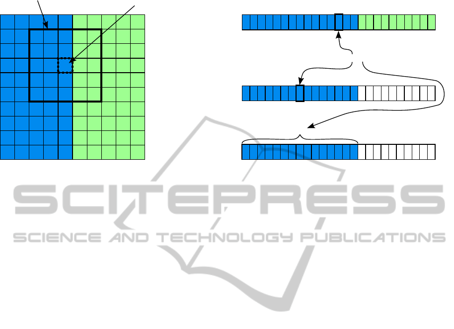
Figure 2: Anisotropic Median Filter: On the left side a simpliﬁed depth map is displayed. The numbers represent the estimated

disparity and the colors indicate the pixel color. Blue pixels are background pixels and green pixels are foreground pixels with

a ground truth of disparity of ”0” and ”1”, respectively. As a consequence blue pixels with a disparity of ”1” are wrongly

estimated due to the fattening effect. The right side shows the working principle of a median ﬁlter, a simple anisotropic

(weighted) average ﬁlter and the anisotropic median ﬁlter for the thick ﬁlter window on the left. While the median would

replace the dotted center pixel with ”1”, the anisotropic median correctly replaces the center pixel disparity with ”0”. The

reason is that it takes only pixels into account that are similar to the center pixel (blue). Although a standard anisotropic

averaging ﬁlter also considers pixel similarity, it fails of returning the correct value of ”0” because it employs no means of

detecting outliers in the disparity values. Thus the ﬁlter result of ”0.33” is contaminated by the outlier values ”1” of the blue

background pixels.

However, for the spatial proximity ∆

(x, p) we rather

apply the Manhattan distance as this can be realized

more efﬁciently than the Euclidean distance on a pixel

grid

∆

( f, p) =

∑

a∈{x,y}

| f

− p

| . (4)

Indeed using the Manhattan distance for spatial prox-

imity corresponds to deﬁning a squared image patch

around a center pixel f. Hence, we will skip ∆

( f, p)

in the following and rather just refer to the size of the

ﬁlter window from which the neighborhood N( f) is

extracted.

Figure 2 displays a simpliﬁed example for visu-

alizing the working principle of the anisotropic me-

dian ﬁlter in comparison to a plain median ﬁlter and a

simple anisotropic averaging ﬁlter. The simple exam-

ple consists of blue background and green foreground

pixels with a ground truth disparity of ”0” and ”1”,

respectively. Some of the blue pixels, however, have

been assigned a disparity ”1” by the stereo algorithm

(fattening effect). By applying a plain median ﬁlter

the wrong disparities are not removed because they

have enough support in the ﬁlter window. In con-

trast, the anisotropic median ﬁlter considers only pix-

els in the ﬁlter window that have a color similar to

the center pixel (blue dotted pixel in Fig. 2). Thus the

wrong disparity ”1” has much less support and the

anisotropic median replaces the center pixel’s dispar-

ity by ”0”. In comparison to this a standard averaging

anisotropic ﬁlter will fail as depicted at the bottom

of Fig. 2. Since all blue pixels get the same weight

the outlier pixels contaminate the ﬁlter result. This is

a typical problem of anisotropic ﬁlters, i.e. disparity

outliers are not considered.

4 COMPUTATIONAL

CONSIDERATIONS

For maps or images which have only a small inte-

ger range the plain median ﬁlter can be calculated

efﬁciently and quasi independently of the ﬁlter size

(Perreault and H´ebert, 2007). Unfortunately, this can-

not be applied to the anisotropic median ﬁlter for dis-

parity reﬁnement. The ﬁrst reason is, that the quasi

size-independent runtime is realized via running his-

tograms. These, however, will get very large for sub-

pixel accurate disparity maps. A second but more se-

vere problem is that due to the anisotropic processing

the neighborhood N(p) of a pixel p cannot be com-

puted by taking the neighborhood N(p − 1) and up-

dating it for pixel p. Because of this the neighborhood

N(p) must be constructed for every pixel (p) indepen-

dently, which also means that the anisotropic median

cannot be calculated in a running ﬁlter fashion.

The na¨ıve approach for ﬁnding the median of a

list of n unsorted elements is to ﬁrst sort the list and

VISAPP2013-InternationalConferenceonComputerVisionTheoryandApplications

192

outlier

removal

hole ﬁlling

anisotropic

median ﬁlter

calculate

disparity map

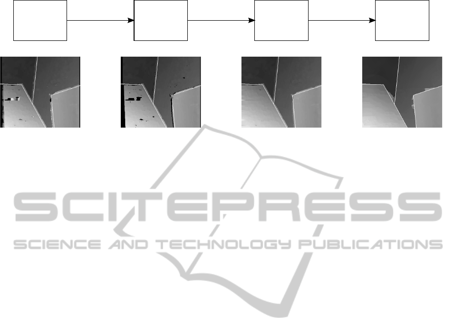
Figure 3: Processing pipeline for anisotropic median ﬁltering. For an optimal result, ﬁrst, outliers have to be removed. The

resulting holes are either ﬁlled by means of applying the anisotropic median exclusively to the holes or by linear interpolation.

Eventually, the anisotropic median is applied to the full disparity map. The white lines in the disparity maps below the ﬂow

chart show the ground truth position of the main depth discontinuities.

then select the median entry. As the best runtime

for any sorting algorithm based on the comparison

of whole keys is bound by Ω(nlog(n)) the na¨ıve me-

dian is bound alike. A better way is to use quicks-

elect (Hoare, 1961). Although this has a worst case

runtime of O (n

) its average runtime is O (n). Since

we apply the anisotropic median on every pixel for

reﬁning a disparity map, the high worst case runtime

has only very little effect. Altogether, applying the

anisotropic median to a whole disparity map has an

expected runtime of O ( ¯nm) with ¯n being the average

neighborhood size and m being the number of pixels

in the disparity map. This means that as long as ¯n is

comparable to the disparity search range d, the run-

time of the anisotropic median is comparable to the

runtime of block-matching stereo which typically has

a runtime of O (dm).

5 PROCESSING PIPELINE

In order to get the best performance of the anisotropic

median (AM) ﬁlter we combine it with means to re-

move outliers from the disparity map. If not re-

moved, outliers that populate the low-texture regions

can hamper the AM ﬁlter. The overall pipeline we

employ is depicted in Fig. 3. For outlier removal we

use a simple technique proposed in (Fua, 1993). The

idea is to remove small areas with constant disparity.

We extend this a bit by removing only those regions

whose disparities differ substantially from the sur-

rounding. It is of course possible to apply also other

techniques like a left-right consistency check (Fua,

1993). In general, it is best to apply such techniques

before the AM ﬁltering. However, in most cases the

removal of the small erroneous areas is sufﬁcient.

As a matter of fact, the outlier removal punches

holes into the disparity map. These holes would lead

to a positive bias in the evaluation, if AM would be

applied directly to the perforated disparity map. The

reason is that the hole pixels are marked with invalid

(negative) disparity values. Thus any estimation of a

real disparity value will be better as the invalid mark-

ing values which will of course reduce the overall dis-

parity error. In order to prevent this bias in the eval-

uation, we apply the AM ﬁlter ﬁrst to the hole pixels

only and consider this as a hole ﬁlling post-processing

step whose resulting disparity map is used as base

line. Since the hole ﬁlling does not alter the other dis-

parity values, the disparity map after the hole ﬁlling

still contains the fattening errors (see Fig. 3).

After the hole ﬁlling step follows the actual AM

ﬁlter step. This is applied to the whole disparity map.

The difference between the disparity error after the

hole ﬁlling step and after the AM ﬁlter step is used for

evaluating our proposed AM ﬁlter in the following.

6 EXPERIMENTS

In this section, we assess the proposed anisotropic

median (AM) ﬁlter by using the Middlebury data set

(Scharstein and Szeliski, 2002). In the ﬁrst experi-

ment, the effectivenessof AM as disparity map reﬁne-

ment is evaluated for different block-matching stereo

approaches. We apply AM to block-matching with

sum of absolute difference (SAD) (Scharstein and

Szeliski, 2002), normalized cross-correlation (NCC)

(Scharstein and Szeliski, 2002), summed normalized

cross-correlation (SNCC) (Einecke and Eggert, 2010)

and rank and census transform (Zabih and Woodﬁll,

1994).

In the following evaluations, the color stereo im-

ages are always transformed to gray level images for

block-matching stereo. Furthermore, rank and cen-

sus require a certain image patch size for transform-

AnisotropicMedianFilteringforStereoDisparityMapRefinement

193

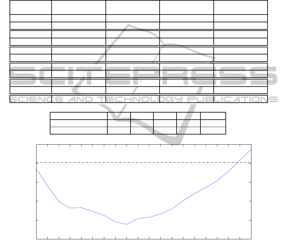
Table 1: Improvement of block-matching stereo by AM post-processing. The block-matching methods used are: sum of

absolute difference SAD (Scharstein and Szeliski, 2002), normalized cross-correlation NCC (Scharstein and Szeliski, 2002),

summed normalized cross-correlation SNCC (Einecke and Eggert, 2010) and rank and census transform (Zabih and Woodﬁll,

1994). The upper table compares the performance of the different methods after the hole ﬁlling step (”+ ﬁll”) and after the

AM ﬁlter step (”+ AM”) (see also Fig. 3). The performance is measured by means of the percentage of bad pixels (Scharstein

and Szeliski, 2002) with a disparity error threshold of 0.5. As the results show, AM leads to an improvement in all cases.

Moreover, the average gain (average difference between the error of ”+ ﬁll” and ”+ AM”) highlights that the improvement is

highest for regions of depth discontinuity. The lower table lists the parameters used for the different block-matching methods.

Tsukuba Venus Teddy Cones

Algorithm nocc all disc nocc all disc nocc all disc nocc all disc

SAD + ﬁll 11.1 12.2 21.3 7.62 8.54 22.8 24.5 30.1 42.7 14.2 21.8 29.5

SAD + AM 8.95 9.61 17.9 3.26 3.73 9.99 21.2 27.0 37.4 10.8 18.0 22.9

RT + ﬁll 10.9 11.8 25.0 4.18 5.13 17.4 13.8 20.8 34.3 7.89 16.0 21.7

RT + AM 9.4 9.9 21.9 1.75 2.32 9.91 12.7 19.8 30.3 7.63 15.1 19.3

NCC + ﬁll 9.84 10.9 24.0 5.03 5.97 21.9 15.7 21.9 37.3 9.16 16.7 23.4

NCC + AM 8.44 9.13 19.5 1.75 2.26 10.2 12.8 18.9 31.3 6.45 13.6 17.7

SNCC + ﬁll 10.3 11.2 21.4 3.44 4.28 14.9 12.3 18.5 30.6 6.11 13.7 16.8

SNCC + AM 9.23 9.89 19.2 1.65 2.08 8.56 11.1 17.2 27.3 5.58 12.8 15.1

Census + ﬁll 11.0 11.7 21.1 3.75 4.61 15.8 12.3 18.7 30.7 6.31 14.0 17.4

Census + AM 9.14 9.60 18.9 1.70 2.18 9.08 11.1 17.2 27.4 6.11 13.2 15.9

average gain 1.60 1.75 3.08 2.78 3.19 9.01 1.94 1.98 4.38 1.42 1.90 3.58

Algorithm SAD RT NCC SNCC Census

block-matching size 7x7 7x7 5x5 5x5 5x5

AM ﬁlter size 21x21 21x21 15x15 17x17 19x19

3 5 7 9 11 13 15 17 19 21 23 25 27 29 31 33 35 37 39 41

10.5

11.5

12.5

AM filter size

bad pixels

Figure 4: This plot shows the performance (bad pixels percentage combined for all four Middlebury scenes) of AM with

respect to its ﬁlter size. The dashed line shows the performance of the census block-matching after the hole ﬁlling step. The

blue, solid line shows the performance after applying AM with different ﬁlter sizes. There are two things to notice. First, over

a large range of ﬁlter sizes the additional application of AM improves the results of the plain block-matching result. Second,

the best AM ﬁlter size of 19x19 pixels is not a strong peak in the error plot. This means that the selection of a good ﬁlter size

for AM is quite stable which is important for a good generalization.

ing the images. Here we use a patch size of 11x11 for

rank transform as proposed in (Einecke and Eggert,

2010) and 7x7 for census transform because this is

the largest odd-valued patch-size that can make use of

the fast 64-bit (Humenberger et al., 2010) processing.

Similarly, we always use a ﬁlter size of 3x3 for the

ﬁrst stage of SNCC as proposed in (Einecke and Eg-

gert, 2010). Furthermore, all used block-matching ap-

VISAPP2013-InternationalConferenceonComputerVisionTheoryandApplications

194

proaches generate sub-pixel accurate disparity maps

by ﬁtting quadratic curves into the matching cost.

For the outlier removal step, we apply a left-right

consistency check and the removal of homogeneous

outlier regions as proposed in (Fua, 1993). The ho-

mogeneous outlier regions are detected by means of

a simple but fast region grouping algorithm. Please

note that the parameters of the outlier removal are

ﬁxed for all block-matching approaches and all ex-

periments.

As described in section 5, we ﬁrst apply the AM

ﬁlter to the invalid hole pixels and consider this as a

hole ﬁlling pre-processing in order to prevent a pos-

itive bias in the evaluation of the performance of the

AM ﬁlter. The invalid hole pixels are marked in the

disparity map by negative disparity values. Therefore

the neighborhood set N( f) for a pixel f needs to be

adapted to consider only pixels with valid disparities

d(p) ≥ 0

N( f) = {p | ∆

( f, p) < θ

∧

∆

( f, p) < θ

∧

d(p) ≥ 0} , (5)

in order to ensure the consistency of the disparity list

D( f). In some cases this can result in very small

neighborhoods N( f) which could lead to wrong re-

sults due to an insufﬁcient statistical signiﬁcance. To

prevent this, we demand the neighborhood N( f) to

have at least a cardinality of nine. If it has a smaller

cardinality, the corresponding pixel f is not processed

by the median ﬁltering, so that the pixel’s disparity is

still invalid. These few remaining hole are ﬁlled by a

simple linear interpolation.

After the disparity maps have been made dense,

the actual AM ﬁlter is applied in a single run to the

whole disparity map for reﬁnement. The reduction in

disparity error by this ﬁnal ﬁlter step is analyzed in

the following.

Table 1 shows the performance of ﬁve different

block-matching approaches right after the hole ﬁll-

ing step and after the AM ﬁlter step of the process-

ing pipeline discussed in Fig. 3. As the different cost

functions have different optimal working parameters

we applied a brute-force optimization to ﬁnd these

points in order to render the different results compara-

ble. The optimal parameters are shown at the bottom

of Table 1. The measure used in Table 1 is the per-

centage of bad pixels as proposed in (Scharstein and

Szeliski, 2002)

∑

|d( f) − GT( f)| > δ , (6)

where δ is the disparity error threshold, d( f) is the

disparity of pixel f and GT( f) its ground truth dis-

parity. In this evaluation we use a threshold of δ = 0.5

to see how well AM can cope with sub-pixel accurate

disparity maps. One might argue that the strong non-

linearity that a median selection involves, destroys the

sub-pixel accuracy of a disparity maps. However, the

results in Table 1 demonstrate that in all cases AM is

able to improve the performance of block-matching

stereo. Hence, it is well suited also for sub-pixel ac-

curate maps. It also strikes that in general the im-

provement for depth discontinuities (disc) is signiﬁ-

cantly larger than for non-occluding regions (nocc) or

the full disparity map (all). This can best be seen in

the average gain which is the average (over all tested

block-matching approaches) error difference between

the ﬁlled disparity maps and the AM ﬁltered dispar-

ity map (see also Fig. 3). The large improvement in

the ’disc’ areas conﬁrms the basic idea behind AM of

reducing the fattening effect. On the other hand, the

improvement for regions without disparity disconti-

nuities reveals that AM surpasses its actual purpose

by providing means for a general disparity map im-

provement.

Figure 4 shows a plot of the disparity error for

different AM ﬁlter sizes applied to the results of the

census block-matching. For comparison the census

performance after the hole ﬁlling step is plotted as a

dashed line. The plot demonstrates two things. First,

over a large range of ﬁlter sizes AM improves the re-

sults of the plain census result. Second, the best AM

ﬁlter size is not a strong peak in the error plot. This

means that the selection of a good ﬁlter size for AM

is quite stable which is important for a good general-

ization.

In order to get a better grasp at the actual improve-

ment capabilities of AM, we compare it in a second

experiment to the local consistency (LC) approach be-

cause LC shares similar characteristics with AM and

it has already proven itself to be very effective. LC is

similar to AM in the following points: First, its pro-

cessing is constrained to local neighborhoods. Sec-

ond, it is non-iterative. Third, it is quite fast with a

runtime of only a few seconds on a standard PC and,

fourth, it has a very small memory footprint.

In this second comparative experiment we use

only SNCC block-matching because it showed the

best overall performance in Table 1 and can thus

be regarded as an upper bound for the other block-

matching approaches. For comparison we use the re-

sults of SNCC that have been reported in the original

paper (Einecke and Eggert, 2010). The authors of that

paper applied a similar outlier removal as we do but

ﬁlled the resulting holes with a depth-discontinuity-

aware linear interpolation. In order to be compara-

ble to (Einecke and Eggert, 2010) we also use a non-

square ﬁlter size of 9x5 for the second stage of the

AnisotropicMedianFilteringforStereoDisparityMapRefinement

195

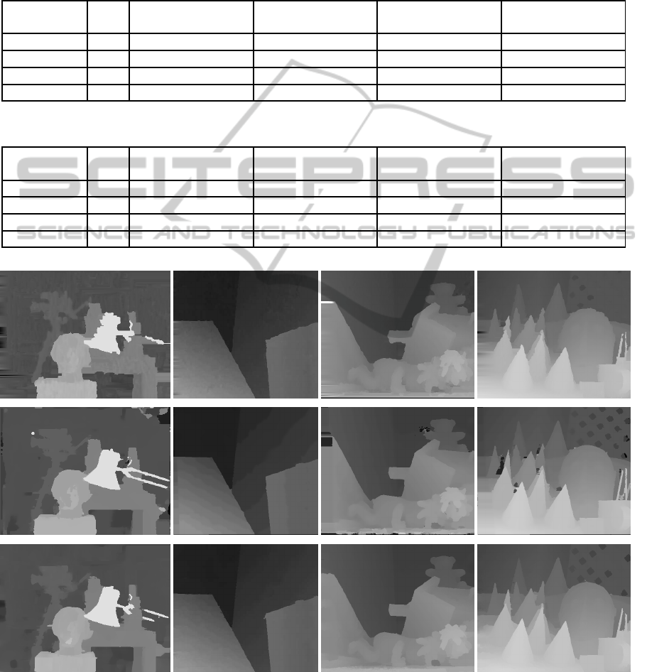
Table 2: Accuracy evaluation according to (Scharstein and Szeliski, 2002) where an error threshold of 0.5 is used for calculat-

ing the bad pixel percentage. The table compares the results of block-matching with SNCC and simple ﬁll-in post-processing

as proposed in (Einecke and Eggert, 2010) against post-processing SNCC block-matching with local consistency LC (Mattoc-

cia, 2009) (SNCC+LC) and the proposed anisotropic median AM ﬁlter (SNCC+AM). The average ranks are taken from the

online Middlebury benchmark at the time of submission (February 2012) to this online benchmark. For further comparison

the then top ranked approach graph-cut + segment border (GC+SB) (Chen et al., 2009) (for δ = 0.5) is also shown. Please note

that SNCC and SNCC+AM compute sub-pixel disparity values while SNCC+LC computes integer disparities. This might

introduce a negative bias for the results of LC in this table. See Table 3 for a comparison with δ = 1.0

avg Tsukuba Venus Teddy Cones

Algorithm Rank nocc all disc nocc all disc nocc all disc nocc all disc

SNCC 25.3 11.3 12.3 27.5 2.35 3.23 15.4 10.6 15.2 28.6 4.71 11.1 13.2

SNCC+LC 13.2 10.3 11.2 16.4 2.14 3.15 9.98 9.56 17.3 24.9 4.46 13.4 10.5

SNCC+AM 10.5 9.96 10.4 19.7 0.76 1.11 6.23 8.70 14.3 23.2 4.47 11.1 12.4

GC+SB 8.6 6.87 7.30 15.3 0.20 0.31 2.44 7.59 9.14 17.5 10.5 11.2 14.4

Table 3: Accuracy evaluation like in Table 2 but with an error threshold of 1.0.

avg Tsukuba Venus Teddy Cones

Algorithm Rank nocc all disc nocc all disc nocc all disc nocc all disc

SNCC 70.6 5.17 6.08 21.7 0.95 1.73 12.0 8.04 11.1 22.9 3.59 9.02 10.7

SNCC+LC 40.5 2.02 2.76 7.76 0.24 1.00 3.39 6.14 14.0 16.3 2.42 10.0 6.32

SNCC+AM 43.4 3.21 3.57 13.6 0.22 0.45 3.01 6.41 10.4 17.7 3.11 8.61 9.27

GC+SB 25.7 1.47 1.82 7.86 0.19 0.31 2.44 4.25 5.55 10.9 4.99 5.78 8.66

Figure 5: From top to bottom: disparity maps generated by block-matching with SNCC + linear interpolation (Einecke and

Eggert, 2010) copied from the Middlebury online database, SNCC + LC and SNCC + AM. Please note that SNCC + linear

interpolation and SNCC + AM compute sub-pixel disparity values while SNCC + LC computes integer disparities.

VISAPP2013-InternationalConferenceonComputerVisionTheoryandApplications

196

SNCC block-matching. Furthermore, we apply LC as

described in (Mattoccia, 2009), i.e. without the pro-

cessing pipeline described in this paper. Again we

optimized the parameters for each approach for com-

parison. For AM we found a ﬁlter size of 19x19

to be most effective and for LC the best parameter

set is R = 39x39, γ

= 31, γ

= 21, γ

= 13, ρ = 40

(please note that this corresponds to the notation used

in (Mattoccia, 2009)).

The results of the comparison of the original

SNCC, SNCC plus LC and SNCC plus AM are shown

in Table 2 and Fig. 5. Again the bad pixel percent-

age with an error threshold of 0.5 is used for this as-

sessment. Furthermore, we used the temporary online

benchmark feature of the Middlebury website to see

how the average rank of the SNCC block-matching

would change in the Middlebury comparison when

applied with the more advanced post-processing of

LC or AM. As can be seen AM and LC improve the

average rank of SNCC from 25.3 to 10.5 and 13.2,

respectively. In fact SNCC+AM achieves overall the

second best result (average rank) behind graph-cut +

segment border (GC+SB) (Chen et al., 2009) in the

Middlebury online benchmark (February 2012) for

δ = 0.5. SNCC+LC would give the third best result.

One reason for the slightly worse results of LC

might be that LC is actually not considering sub-pixel

accuracies. In order to test this hypothesis Table 3

shows the performance for a disparity error thresh-

old of 1.0. Indeed, the results in Table 3 demonstrate

that LC is slightly better than AM for this less strict

threshold. Thus, one can conclude that overall LC

and AM show a very similar performance but that AM

is more advantageous for sub-pixel accurate disparity

maps while LC is more accurate for integer-valued

disparity maps.

6.1 Runtime

The runtime of AM is about 850ms for the teddy

scene on one core of an Intel Core i5 with 3.2GHz.

Considering that fast block-matching takes around

150ms (Einecke and Eggert, 2010; Humenberger

et al., 2010) for the teddy scene, AM is too slow for

a realistic real-time application on a mobile system.

In order to improve this, we apply a sparseness tech-

nique described for the census transform in (Humen-

berger et al., 2010). Instead of calculating the me-

dian of the whole neighborhood, only pixels in ev-

ery second row and column are used, i.e. only one

fourth of all neighborhood pixels are evaluated. By

doing so the runtime decreases to 270ms with a small

degradation of the result to an average rank of 12.2

which is still the second best result (February 2012)

for δ = 0.5. Hence, the sparse anisotropic median

allows for a time efﬁcient post-processing of block-

matching approaches.

7 SUMMARY AND DISCUSSION

In this paper, we presented the anisotropic median

(AM) ﬁlter, a novel technique for disparity map post-

processing with a focus on the reduction of the fat-

tening effect. The main application we have in mind

for this post-processing are block-matching generated

disparity maps because these are prone to the fatten-

ing effect. The basic idea is to extend the standard me-

dian ﬁlter by taking only pixels into account that are

similar to the center pixel of the ﬁlter window. Due to

this, disparity values that are inconsistent with similar

pixels are replaced by consistent ones. This consti-

tutes an anisotropic smoothness constraint that is ap-

plied to the disparity map. Experiments with block-

matching stereo and different cost functions demon-

strated that in all cases AM leads to a signiﬁcant im-

provement of the quality. Furthermore, a comparison

with state-of-the-art methods for disparity map reﬁne-

ment shows that AM has a comparable performance

but at a much lower computational cost. In fact,

we could demonstrate that AM applied to disparity

maps of block-matching stereo with summed normal-

ized cross-correlation achieves the second best rank-

ing (February 2012) in the Middlebury stereo bench-

mark (δ = 0.5) with a total processing time (block-

matching plus AM) of 420ms on a single CPU core.

This highlights that real-time and accurate stereo is

possible with restricted resources as commonly found

on mobile robots and platforms.

We identiﬁed some issues of AM that need to

be tackled in future work. Currently, we use a sim-

ple region detection method to remove outlier regions

that might negativelyinﬂuence the performance of the

AM ﬁlter. Although this worked reliably with a ﬁxed

parameter setting in our experiments, it is not guaran-

teed to work in general. Hence, it would be prefer-

able to replace this with a more concise technique.

Second, the used Euclidean distance over RGB val-

ues is known to be a weak color similarity measure.

For future investigations it is important to test and

compare other color spaces. Third, our experiments

involved mainly stereo data with colorful scenes. It

has to be analyzed in future work how the AM ﬁl-

ter is coping with less saturated and monochromatic

images. This is especially important for real-world

applications where the images typically exhibit only

weak color contrasts. Fourth, the speed of AM is not

fully satisfying yet. Further strategies have to be in-

AnisotropicMedianFilteringforStereoDisparityMapRefinement

197

troduced before AM is really applicable to real-time

mobile robotic systems. One way to reduce the com-

putational cost is to use only one of the RGB color

channels or the hue channel of the HSV space or just

gray-level images. However, as discussed above this

might reduce the accuracy. On the other hand, AM is

currently using the pixel color information of one im-

age only. A symmetric approach as proposed in (Mat-

toccia, 2009) could further improve accuracy, how-

ever, at the cost of an increased computational effort.

This means one goal of the future work is also to op-

timize the different processing alternatives for a good

trade-off between speed and accuracy.

ACKNOWLEDGEMENTS

The authors would like to thank Stefano Mattoccia

from Dipartimento di Elettronica Informatica e Sis-

temistica (DEIS) of the University of Bologna for

applying his local consistent stereo method to our

SNCC data for comparison.

REFERENCES

Banno, A. and Ikeuchi, K. (2009). Disparity map reﬁnement

and 3D surface smoothing via directed anisotropic dif-

fusion. In 3DIM Workshop, pages 1870 – 1877.

Chen, W., Zhang, M., and Xiong, Z. (2009). Segmentation-

based stereo matching with occlusion handling via re-

gion border constrains. CVIU.

Einecke, N. and Eggert, J. (2010). A two-stage correlation

method for stereoscopic depth estimation. In DICTA,

pages 227–234.

Fua, P. (1993). A parallel stereo algorithm that produces

dense depth maps and preserves image features. Ma-

chine Vision and Applications, 6(1):35–49.

Heo, Y. S., Lee, K. M., and Lee, S. U. (2008). Illumination

and camera invariant stereo matching. In CVPR, pages

1–8.

Hirschm¨uller, H. (2005). Accurate and efﬁcient stereo pro-

cessing by semi-global matching and mutual informa-

tion. In CVPR, pages II: 807–814.

Hoare, C. A. R. (1961). Algorithm 65: Find. Communica-

tion of the ACM, 4(7):321–322.

Humenberger, M., Zinner, C., Weber, M., Kubinger, W.,

and Vincze, M. (2010). A fast stereo matching algo-

rithm suitable for embedded real-time systems. CVIU,

114(11):1180–1202.

Lucas, B. D. and Kanade, T. (1981). An iterative image

registration technique with an application to stereo vi-

sion. In IJCAI, pages 674–679.

Matthies, L., Kanade, T., and Szeliski, R. (1989). Kalman

ﬁlter-based algorithms for estimating depth from im-

age sequences. IJCV, 3(3):209–238.

Mattoccia, S. (2009). A locally global approach to stereo

correspondence. In 3DIM Workshop, pages 1763–

1770.

Mattoccia, S. (2010). Fast locally consistent dense stereo

on multicore. In ECVW, pages 69–76.

Perona, P. and Malik, J. (1990). Scale-space and edge detec-

tion using anisotropic diffusion. IEEE Trans. Pattern

Anal. Mach. Intell., 12(7):629–639.

Perreault, S. and H´ebert, P. (2007). Median ﬁltering in con-

stant time. IEEE Transactions on Image Processing,

16(9):2389–2394.

Scharstein, D. and Szeliski, R. (2002). A taxonomy and

evaluation of dense two-frame stereo correspondence

algorithms. IJCV, 47(1-3):7–42.

Sun, D., Roth, S., and Black, M. J. (2010). Secrets of optical

ﬂow estimation and their principles. In CVPR, pages

2432–2439.

Sun, X., Mei, X., Jiao, S., Zhou, M., and Wang, H. (2011).

Stereo matching with reliable disparity propagation.

In 3DIMPVT, pages 132–139.

Tian, Q. and Huhns, M. N. (1986). Algorithms for subpixel

registration. CVGIP, 35(2):220–233.

Wang, L., Liao, M., Gong, M., Yang, R., and Nister, D.

(2006). High-quality real-time stereo using adap-

tive cost aggregation and dynamic programming. In

3DPVT, pages 798–805.

Yang, Q., Yang, R., Davis, J., and Nist´er, D. (2007). Spatial-

depth super resolution for range images. In CVPR,

pages 1–8.

Yoon, K.-J. and Kweon, I. S. (2006). Adaptive support-

weight approach for correspondence search. IEEE

Trans. Pattern Anal. Mach. Intell., 28:650–656.

Zabih, R. and Woodﬁll, J. (1994). Non-parametric local

transforms for computing visual correspondence. In

ECCV, pages 151–158.

VISAPP2013-InternationalConferenceonComputerVisionTheoryandApplications

198

REFERENCES

Banno, A. and Ikeuchi, K. (2009). Disparity map refinement