
Planning and Control Model for a Forest Supply Chain
C. Alayet
1, 3
, N. Lehoux
1, 3
, L. Lebel
2, 3
and M. Bouchard
4
1
Department of Mechanical Engineering, Laval University, Quebec, Canada
2
Department of Wood Science and Forest, Laval University, Quebec, Canada
3
Interuniversity Research Centre on Enterprise Networks, Logistics and Transportation, Quebec, Canada
4
NSERC VCO Network, University Laval, Quebec, Canada
Keywords: Decision Making Process, Forest Industry, Mixed-Integer Linear Model, Logistics Planning.
Abstract: This paper presents a mixed-integer linear program (MILP) for a planning problem of multiple activities in
the forest industry. The model developed aims at maximizing the total profit of the value chain by
optimizing operations in harvesting, transportation, storage, and production. The main motivations for the
model is a need to better account for important factors in planning and control, such as quality, freshness,
and species of wood products. These factors have a direct influence on costs and supply decisions. In
particular, the model developed will improve forest product companies’ industrial processes by a better
control over the wood fibre freshness. Furthermore, our model is designed for a context where multiple
independent companies supply their raw material from the same sources. It can therefore be used as a
support tool for collaboration between actors in a forest supply chain.
1 INTRODUCTION
The forest industry is an important economic sector
for Canada. In 2011, it provided a value of $ 26.0
billion of Canada’s total export with a gross
domestic product of $ 23.2 billion. Therefore it
ensures about 600,500 direct and indirect
employments (
FPAC, 2011).
However, the forest industry network is complex,
being composed of a set of nodes (i.e., forest,
sawmills, paper mills, wholesalers, retailers …)
interconnected by flows of materials (i.e., logs,
chips, lumber, paper …), information (orders,
demand, forecasts …), and financial transactions.
The network also includes a large set of constraints,
for example those related to product quality (for
lumber, paper, and other forest products), raw
material availability, and capacity requirements (at
the different business unit sites). Among these
constraints, product quality has reached standards
that require a very precise control over the supply
and production processes. For forest products,
freshness of raw material such as the logs and wood
chips is considered essential to optimise value while
satisfying customer needs. Furthermore, as a general
rule, the lower the quality of the fibre, the higher the
production cost for manufacturing forest products
(Beaudoin et al., 2006); (Maness and Norton, 2002).
In order to improve its efficiency, the forest
supply chain needs a continuous supply of raw
materials to ensure quality and achieve expected
standards. On the other hand, the procurement of
timber is a real challenge because of the fibre quality
variation, especially in the presence of various forest
stands and many tree species. The problem becomes
even more complex when many independent firms
in the same region use wood from the same stands to
produce their forest products. If each firm plans its
own activities without considering the needs of the
others (e.g., small or large trees, fir or spruce ...), the
wood fibre will not necessarily be matched to mill
demands efficiently. Moreover, the residue of one
company (i.e., chips from sawmill) becomes the raw
material for another one (i.e., the paper mill).
Therefore when there is no coordination between
the stakeholders, it leads to a set of problems such as
higher stock levels in the forest or at the different
business unit sites, delivery times not respected,
unsatisfied demands, poor value of the final product,
and so on. From operational and tactical planning
perspectives, timber supply is challenging on several
levels. it involves several activities such as forest
road building and maintenance, selection and
scheduling of harvesting areas, transport operations
(truck routing and scheduling), and the coordination
of interactions between these activities based on
203
Alayet C., Lehoux N., Lebel L. and Bouchard M..
Planning and Control Model for a Forest Supply Chain.
DOI: 10.5220/0004202200050013
In Proceedings of the 2nd International Conference on Operations Research and Enterprise Systems (ICORES-2013), pages 5-13
ISBN: 978-989-8565-40-2
Copyright
c
2013 SCITEPRESS (Science and Technology Publications, Lda.)

information sharing. Resolving these issues may be
achieved through planning and effective monitoring
of resource flows and improved business processes
in a network of value creation (Suzanne et al., 2004).
The present work aims at helping forest companies
in better planning and controlling their forest supply
activities through a mathematical model that could
be used as a decision support tool for value creation.
The main motivation of the model is to deal with
elements of competition namely cost, quality, and
agility. More specifically, the model developed aims
at optimizing all activities related to the satisfaction
of customer demand, that is the quantity of wood to
harvest and to transport to the sawmills, the quantity
of lumber and chips to produce, the paper needed to
satisfy the demand, and the different products to
keep in stock to ensure a certain level of service. To
achieve these results, we assume that there is no
competition between the different business units.
Diverse scenarios are also tested to evaluate the
impact of wood freshness variations, price changes,
and demand variations on the value network. These
scenarios were explored to reflect the reality of the
forest industry.
The paper is structured as follows: the next
section presents a literature review, followed by the
description of the case study. Section 4 describes the
modelling of the problem and the assumptions made.
The experiment is then explained in detail in Section
5. Finally, Section 6 concludes the paper.
2 LITERATURE REVIEW
Managing the forest supply chain is an important
activity due to its impact on value creation and the
generation of profits for all business units. It
involves different planning decisions that should
cover different levels: strategic, tactical, and
operational (Martel, 2003). It begins with the
harvesting of wood in the forest, followed by species
sorting, wood transportation to different mills, log
sawing, and processing factories such as pulp, paper,
and energy. It ends with the delivery of final forest
products to end users (Carlsson et al., 2006).
However, planning decisions and their optimization
are complex tasks since they have to include many
factors such as wood species, wood freshness,
lumber price, final product quality, processing time,
and so on, as well as multiple independent decision-
makers.
Therefore, different planning approaches have
been proposed over the time to better use the wood
fibre and ensure the synchronization of network
activities. Beaudoin et al., (2010) presented supply
planning models for multiple forest companies in
which supply areas are shared. These planning
models were based on coordination and
collaboration approaches coupled with distributed
and centralized structures. Horne et al., (2006)
explained the importance of value creation based on
innovation and the development of products and
processes from a center of expertise in the forest
industry. The objective of their research was to
develop a model based on value creation of
innovative knowledge to improve decision making
and facilitate understanding of complex
mechanisms.
It is difficult to think about planning forest
operations without considering the control of the
different logistic activities. In the literature, there are
many definitions of logistic control systems. Among
them, we evoke the definition of Meinadier (1998)
cited in Trentesaux and Tahon (2010). The authors
introduced three activities that defined the driving
process: capture, edit, and order.
Several control structures were used to solve
complex problems of the forest supply chain. We
first distinguish the centralized or integrated
structure. This is the classic approach in which all
resources are controlled by a single decision center.
This center oversees the supply chain, synchronizes
and coordinates the various resources, and manages
real-time contingencies that occur (Mirdamadi et al.,
2009). Among the works that rely on a centralized
control structure, we find the work of Walker and
Preiss (1988). They developed a model for planning
logging (harvesting, quantity of timber harvested per
block, etc.) and transportation activities.
A second approach is characterized by a
coordinated structure. This structure aims at
ensuring coordination between the subsystems and
improving resource utilization while promoting a
better flow of information (Martel, 2003). This
structure usually improves the ability of decision in
each sub-control system to effectively solve
problems (Mirdamadi et al., 2009). It is within this
context that the study of D'Amours et al., (2004)
mentioned the importance of coordination in
establishing a value forest product network. The
authors identified four dimensions for this structure:
(1) competitiveness and customer service, (2)
integration, (3) coordination, and (4) operational
excellence.
Several other driving approaches were treated in
the literature depending on the area of study as well
as the planning horizon aimed, such as the
distributed approach (Gaudreault et al., 2009), the
ICORES2013-InternationalConferenceonOperationsResearchandEnterpriseSystems
204
hierarchical approach (Chang et al., 2009), etc.
However, the lack of collaboration between network
members is a major obstacle for planning and
controlling logistic activities efficiently (Lehoux et
al., 2008). In the forestry context, few authors
treated the topic of collaboration. Beaudoin et al.,
(2010) used a MILP approach and protocols of
negotiation / collaboration to plan the wood supply
for multiple forest companies. Lehoux et al., (2011)
evaluated various collaborative strategies between a
pulp and paper producer and its customer. They
presented different MILP models as well as a
methodology to solve the various modes of
collaboration and measure their impact on partners’
benefits.
The different articles show that forest supply
chain optimization has an increasing interest, the
planning of the different activities and the
integration of many factors such as quality
representing real challenges. This context will
therefore be explored in the following section.
3 CASE STUDY
3.1 Problem Description
The effective management of the forest supply chain
certainly requires a better planning and control of
logistic activities. Nevertheless, the management of
material flows and information is considered
complex, because of the interdependence of the
stakeholders involved, the quantity and the quality
of the information needed, and success factors such
as demand satisfaction and product quality.
Moreover the freshness of the wood fibre is a
particular problem that characterizes the forest
product market. It influences the harvesting
decisions like labor allocation, harvesting schedules,
site selection, etc. Similarly, the wood freshness
often causes problems during processing operations
such as the choice of the technology and the way to
use this technology (sawing processes, parameters
setting and cutting setup times for sawmills, etc.).
Thus, the freshness of the raw material has a
direct effect on the manufacturing process, the plant
performance, and the quality of finished products. In
the pulp and paper industry, the chips freshness has
a direct impact on the quantity of chemical products
(whiteness) to be added during the production.
Solving the above enumerated problems represents
long, medium, and short term decisions that have a
direct influence on production costs.
In this context, we study the case of a forest
supply chain located in Côte-Nord, a Quebec region
in Canada. The network includes several harvesting
areas, covering 103,146 km2 while 84,382 km2 are
accessible and productive forest lands (MRNFP,
2004). Several sawmills with variable processing
capacities procure their raw material/logs/timber
from these harvesting areas. The wood is used to
manufacture lumber for construction market as well
as chips delivered to a pulp and paper mill located in
the same region. In recent years, the network has
faced many difficulties such as an overcapacity of
sawing, a decrease in wood fibre quality, and higher
operational costs. Combined with a lower demand
for forest products on traditional markets, these
factors lead to a loss of 6,300 jobs in the last five
years. Different studies suggested that procurement
cost could be reduced and final product quality
increased if raw material quality could be better
matched to mill demands. To make this possible, a
global strategy involving a better planning and
control over the network activities is required.
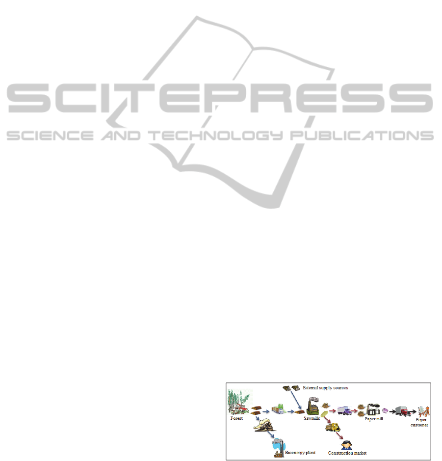
To address this challenge, we have first
developed an integrated or centralized planning
model adapted to this context. The model includes
five forest areas and the four sawmills of the region.
A fictional bioenergy plant has been added because
the region is considering using wood residues for
energy. The forest is made up of two different
species, fir and spruce, and four intermediate
products are delivered to the sawmills (small and
large spruce logs + small and large fir logs).
Sawmills can also be supplied from external sources
to cover the lack in case of high demand. Sawmills
consume raw material to produce chips for paper
making as well as lumber for the construction
market. The model also takes into account a paper
mill supplies by the four sawmills. The paper mill
gets all its chips from the sawmills. It produces
newsprint and magazine paper.
The main objective of this study is to determine
an effective supply plan for this network that could
maximize the profit of all the stakeholders. An
illustration of the network is given in Fig 1.
Figure 1: Logistics network of the case study.
PlanningandControlModelforaForestSupplyChain
205

3.2 Assumptions
The model developed is based on a one-year
planning period divided into fifty-two weeks. Our
experiment is performed on a rolling horizon of four
weeks (Fig. 2). For each scenario, we solve the
model for the first four weeks, for example weeks 1
to 4. Then, we consider the results of the first week
to solve the next four weeks, weeks 2 to 5, and so
onBy using a rolling horizon, we can develop a 4
week schedule for forest operations while
considering updates, revisions, and adjustments
when necessary. This assumption has been made to
reflect companies’ reality.
Figure 2: An example of the rolling horizon approach
used.
We also assume that the level of freshness of the
wood fibre is divided into three categories: green
(young or fresh), yellow (medium or less fresh), and
red (old or not fresh).
In particular, we use "θ" to reflect the percentage
of aging during the period "t", and these parameters
are set according to product types and seasons.
Furthermore, φ is the percentage of aging per time
unit. So if the percentage of aging per week, θ, is
seven days, the percentage of aging per day is:
φ =
√
7
(1)
4 MATHEMATICAL
MODELLING
In this section, the mathematical model for Côte-
Nord network is presented. The model, based on a
centralized driving approach, reflects the network
shown in Figure 1.
Through this model, we try to maximize profits
for forest companies by determining harvested
volumes, the quantities to keep in stock and to
transport at each node, as well as the quantities
produced by the processing units. The decision
variables, parameters, and the complete
mathematical model are described in Appendix A.
The objective function is summarized by equation
(2).
(2)
Where R is the revenue of the value network, C
, the
cost for harvesting operations, C
,the cost for
buying wood from an external supply, C
, the total
transportation cost (transport between network
nodes: forest, plants, and customers), C
, the
inventory cost for the whole network, and C
,the
cost for processing the wood at the different
business units.
The network revenues are generated from the
sale of lumber, paper and the delivery of wood
residues to the bioenergy plant. Costs are divided
into several categories. Specifically, the harvesting
cost includes the cost for forest road construction
and maintenance, as well as the administrative cost.
The cost of external supply includes all costs
induced by moving logs from an outside supplier to
the sawmill (purchasing cost, ordering cost …). The
transportation cost includes product delivery costs as
well as loading and unloading costs. There is also an
inventory cost that includes, among other things,
material handling and equipment costs. The
processing cost then covers the costs and expenses
for producing lumber, wood chips, and paper.
As presented in detail in Appendix A, constraints
have been defined to represent the Côte-Nord
context. Two constraints were used to ensure
customer demand satisfaction. Two other constraints
have been added to ensure a product flow balance
between the sawmills and the paper mill. In order to
reflect aging at the different storage areas (i.e.,
forest, sawmills and paper mills sites), different
constraints were used. Constrains for processing
capacity of each business unit, capacity of the
different storage areas, and transportation capacity
were also considered. Finally, a constraint has also
been used to specify the maximum capacity of
supply from external sources.
5 EXPERIMENTATION AND
DISCUSSION
5.1 Scenarios and Results
The mathematical model was solved using the
CPLEX solver under ILOG OPL environment.
Several scenarios were tested to solve the problem.
First, different levels of freshness were considered in
ICORES2013-InternationalConferenceonOperationsResearchandEnterpriseSystems
206
order to evaluate its effect on network profits.
Demand variability was also taken into account to
reflect the reality of the forest industry. A
disturbance of market prices for lumber was then
analyzed because the price for forest products is
usually far from linear so it becomes necessary to
understand the impact of this change on the system.
If we look at the first scenario, five levels of wood
freshness have been explored. The percentage of
aging assumed for each level is presented in Table 1.
Table 1: Levels of wood freshness considered in the
experimentation.
Levels 1 2 3 4 5
(%)
0 10 30 50 60
Results summarized in Table 2 show that a
decrease in fibre quality (freshness) has a direct
impact on the total network profit.
Table 2: Results for variations of wood freshness.
Costs (M $) \
Instances
1 2 3 4 5
Harvest Cost 861.3 861.5 852 801.1 751.9
Cost of
External
Supply
268.7 265.8 272.4 317 392.4
Storage Cost 31.5 32 33.1 36.1 40.9
Total Cost 1953.6 1950.3 1945.2 1931.4 1972.6
Revenue 2055.6 2052.2 2050 2039.3 2051.7
Network
profit
102 101.9 104.8 107.9 79.1
We also note an improvement in profit when
some of the forest products become older from one
period to another. This improvement is justified by
the demand for products of lower quality that
necessarily cost less to the customer and that cannot
be satisfied when all the wood fibre is considered
fresh. However, it is clear that when the percentage
of aging is very high (i.e., 60%), the network profit
decreases abruptly. Indeed, the rapid aging forces
sawmills to buy wood from external supply sources
which significantly increases the cost of external
supplies. We can also point out the storage cost that
becomes more and more significant. This increase is
justified by the accumulation of low quality wood
fibre that remains in stock from one period to
another. This inventory cost will therefore decrease
the total profit. Similarly, the cost for harvesting and
logging significantly decreases when the percentage
of aging increases. In fact, when there is a rapid
aging, the network optimization requires a decrease
of harvesting because the harvested logs quickly get
old and remain in storage due to low demand for low
quality.
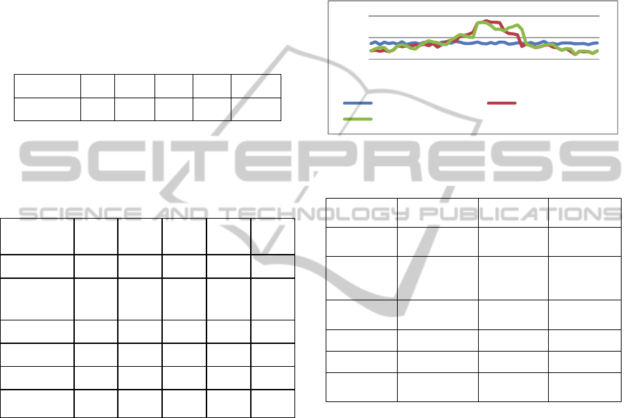
The second scenario considered different
variations of the lumber demand, that is, few
perturbations, seasonality, and cyclical seasonality
(Fig 3).
Figure 3: Variations of the lumber demand (m
3
/Week).
Table 3: Results for variations of the lumber demand.
Costs (M $)
\ Instances
Few
perturbations
Seasonality
Cyclical
seasonality
Harvest
Cost
873.0 867.9 875.2
Cost of
External
Supply
250.3 252.1 254.3
Storage
Cost
31.8 30.6 30.4
Total Cost 1945.6 1934.7 1947.1
Revenue 2080.5 2035.4 2050.5
Network
profit
134.9 100.7 103.4
The benefits of having a stable timber demand
are highlighted by Table 3. In fact, stability is
difficult to achieve since demand for lumber, at least
in Canada, is characterized by a seasonal structure
related to the construction market. To ensure a more
constant demand, forest product companies are
therefore trying to develop new external markets by
producing more value-added products.
Results in table 3 show that the harvesting cost is
lower when the demand is seasonal. This is due to
the fact that it is cheaper to harvest during the
summer (favorable climatic condition). The cost
related to external supplies is also not negligible,
since it represents almost a quarter of the total cost.
This value is justified by a harvesting capacity that is
limited and even null during the thawing season.
The sale price is an important and a classic factor
to consider in the analysis of a value creation
network. For our case study, results show that the
network profit may be doubled if the lumber price
750
950
1150
1 142740
Few perturbations Seasonality
Cyclical seasonality
PlanningandControlModelforaForestSupplyChain
207

increases by 7%. These results are justified by the
importance of lumber demand that represents almost
80% of the total network demand. Thus, it becomes
essential to plan the supply chain efficiently in order
to deliver the right product to the right customer
with the right quality. By managing quality
standards (freshness) it becomes also possible to
offer a more advantageous and stable price.
6 CONCLUSIONS
This article proposes an integrated model to plan
supply chain operations for the forest industry while
considering key constraints related to the freshness
of the wood fibre. In particular, we analyze a case
study, which includes four sawmills and one paper
mill located in eastern Canada. To ensure a better
use of the wood fibre and a greater synchronization
of the network activities, the model provides
harvesting, transportation, production, and storage
plans for the forest companies of this region. The
model aims at improving the management of the
wood fibre quality while reducing the operating
costs such as storage, transportation, and processing.
The proposed model has been tested using three
different scenarios: variations of the wood freshness,
different patterns of lumber demand, and variations
of the lumber price. Results show that the wood
fibre freshness is a key criterion to consider for
increasing the benefit of the value network. On the
other hand, scenario analysis based on lumber price
and demand confirm the necessity for Canadian
forest product companies to expand their market to
avoid the effects of the relative instability of the
Canadian lumber market.
The next step will be to develop multiple models
based on a coordinated driving strategy for
addressing the fact that each company is
“independent” or autonomous. It will also be
necessary to develop some mechanisms to ensure a
fair benefit sharing generated of a better
synchronization of network members’ operations.
REFERENCES
Beaudoin, D., Frayret, J. M., LeBel, L., 2010. Negotiation-
based distributed wood procurement planning within a
multi-firm environment. Forest Policy and Economics,
vol. 12, no. 2, pp. 79–93.
Beaudoin, D., LeBel, L., Frayret, J. M., 2006. Tactical
Supply Chain Planning and Robustness Analysis in the
Forest Products Industry. Canadian Journal of Forest
Research, vol. 37, no. 1, pp. 128-140(13).
Carlsson, D., D'Amours, S., Martel, A., Rönnqvist, M.,
2006. Supply Chain Management in the Pulp and
Paper Industry. CENTOR, Working Paper, DT-AM-3.
Chang, Y. H., Weyb, W. M., Tseng. H. Y., 2009. Using
ANP priorities with goal programming for
revitalization strategies in historic transport: A case
study of the Alishan Forest Railway. Expert Systems
with Applications, vol. 36, no. 4, pp. 8682–8690.
D’Amours, S., Frayret, J. M., Rousseau, A., 2004. De la
forêt au client – Pourquoi viser une gestion intégrée
du réseau de création de valeur ? Université Laval,
FORAC, CENTOR, Document de travail.
Forest Products Association of Canada (FPAC)., 2011.
Industry by the number. Key economics facts.
Gaudreault, J., Frayret, J. M., Pesant, G., 2009. Distributed
search for supply chain coordination. Computers in
Industry, vol. 60, no. 6, pp. 441–451.
Horne, C. V., Frayret, J. M., Poulin, D., 2006. Creating
value with innovation: From centre of expertise to the
forest products industry. Forest Policy and
Economics,vol. 8, no. 7, pp. 751–761.
Lehoux, N., D’Amours, S., Langevin, A., 2008.
Collaboration et coordination dans les réseaux, une
revue des travaux clés. CIRRELT-2008-51.
Lehoux, N., D’Amours, S., Frein, Y., Langevin, A., Penz,
B., 2011. Collaboration for a two-echelon supply
chain in the pulp and paper industry: the use of
incentives to increase profit. Journal of the
Operational Research Society, vol. 62, pp. 581-592.
Maness, T. C., Norton, S. E., 2002. Multiple Period
Combined Optimization Approach to Forest
Production Planning. Scandinavian Journal of Forest
Research, vol. 17, no. 5, pp. 460-471.
Martel, A., 2003. Le pilotage des flux : concepts de base et
approches contemporaines. DF-3.1.1. La conception
de réseaux logistiques. CENTOR, Université Laval.
Ministère des ressources naturelles, de la faune et des
parcs, direction régionale de la Côte-Nord (MRNFP).,
2004. Région de la Côte-Nord. Document
d’information sur la gestion de la forêt publique.
Mirdamadi, S., Dupont, L., Fontanili, F., 2009.
Modélisation du processus de pilotage d’un atelier en
temps réel à l’aide de la simulation en ligne couplée à
l’exécution. Thèse de doctorat. Institut National
Polytechnique de Toulouse.
Suzanne, T., Roy, D. S., Ari-Pekka, H., 2004. From supply
chain to demand chain: the role of lead time reduction
in improving demand chain performance. Journal of
Operations Management, vol. 21, no. 6, pp. 613–627.
Trentesaux, D., Tahon, T., 2010. Pilotage hétérarchique
des systèmes de production. Habilitation à diriger des
recherches. L’Université de Valenciennes et du
Hainaut-Cambresis. LAMIIH. UMR CNRS 8530.
Walker, H. D., Preiss, S. W., 1988. Operational planning
using mixed integer programming. The Forestry
Chronicle, vol. 64, no. 6, pp. 485-488.
ICORES2013-InternationalConferenceonOperationsResearchandEnterpriseSystems
208

APPENDIX
The data required to formulate the problem are:
r: Set of products
w: set of supply sources
e: Set of external supply sources
u: Set of sawmills
u’: Other Plants (bioenergy plant ...)
u’’: Set of paper mills
c: End clients of paper mills
b: Timber clients
a: Level of freshness (age group: 1: green (young),
2: yellow (medium), 3: Red (old))
t: Number of periods
The decision variables, parameters and coefficients
used for mathematical modeling are:
Parameters
C
: Unit harvesting cost of product r belongs to
the supply source w during period t
C
: Unit supply cost of product r from external
supply source e to the plant u’ during period t
C
: Unit storage cost of product r in the supply
source w during period t
C
: Unit transporting cost of product r from the
source w to the sawmill u during period t
C
: Unit transporting cost of product r from the
source w to the plant u’ during period t
C
: Unit transporting cost of product r from the
sawmill u to the paper mill u’’ during period t
C
: Unit transporting cost of product r from the
sawmill u to the timber client b during period t
C
: Unit storage cost of raw materials r in the
sawmill u during period t
C
: Unit storage cost of raw materials r in the
paper mill u’’ during period t
C
: Unit storage cost of finished product r in the
sawmill u during period t
C
: Unit storage cost of finished product r in the
paper mill u’’ during period t
C
: Unit production cost of product r, aged a, in
the sawmill u during period t
C
: Unit production cost of product r, aged a, in
the paper mill u during period t
p
: Selling price of product r, aged a and directly
transported to the plant u’ during period t
p
: Price of finished product r, aged a and
manufactured by the sawmill u during period t
p
: Price of finished product r, aged a and
produced by the paper mill u during period t
α
: Coefficient of adjustment of units: raw material;
finished product r for the sawmill u
β
: Coefficient of adjustment of units: raw
material; finished product for the paper mill u’’
θ
: Proportion of aging product r, aged a for the
source w
θ
: Proportion of aging product r, aged a for the
initial stock of the sawmill u
θ
: Proportion of aging product r, aged a for the
final stock of the sawmill u
θ
: Proportion of aging product r, aged a for the
initial stock of the paper mill u’’
θ
: Proportion of aging product r, aged a for the
final stock of the paper mill u’’
b
: Maximum harvesting capacity product r of the
source w during period t
b
: Minimum harvesting capacity product r of the
source w during period t
b
: Maximum available storage capacity of the
supply source w
b
: Maximum storage capacity for raw materials
from the sawmill u
b
: Maximum storage capacity for raw materials of
the paper mill u’’
b
: Maximum storage capacity of finished products
from the sawmill u
b
: Maximum storage capacity of finished products
of the paper mill u’’
b
: Maximum transport capacity from the source w
during period t
b
: Minimum transport capacity from the source
w during period t
b
: Maximum supply capacity from the external
source e during period t
b
: Maximum transport capacity from the sawmill u
during period t
b
: Maximum processing capacity of the sawmill u
during period t
b
: Maximum processing capacity of the paper
mill u’’ during period t
D
: Demand of product r, aged a, from the
sawmill u customers during period t
D
: Demand of product r, aged a, from the paper
mill u’’customers during period t
M: Big number
Decision Variables
: Harvested volume of product r from the source
w during period t
: Stored volume of product r, aged a, in the
supply source w during period t
: Transported volume of product r, aged a,
from the source w to the sawmill u during period t
PlanningandControlModelforaForestSupplyChain
209

: Transported volume of product r, aged a,
from the source w to the plant u’ during period t
: Transported volume of product r, aged a,
from the external source e to the plant u’ during
period t
: Transported volume of product r, aged a,
from the sawmill u to the paper mill u’’ during
period t
: Transported volume of product r, aged a,
from the sawmill u to the timber client b during
period t
: Transported volume of product r, aged a,
from the paper mill u’’ to the final client c during
period t
: Inventory of stored raw materials r, aged a,
in the sawmill u during period t
: Stored volume of final product r, aged a, in
the sawmill u during period t
: Inventory of stored raw materials r, aged a,
in the paper mill u’’ during period t
: Stored volume of final product r, aged a, in
the paper mill u’’ during period t
: Inventory volume of transformed product r,
aged a, in the sawmill u during period t
: Quantity of available finished products r,
aged a, in the sawmill u during period t
′′
: Quantity of available finished products r,
aged a, in the paper mill u during period t
′′
: Inventory volume of transformed product r,
aged a, in the paper mill u’’ during period t
: 1, if the source w is transported to the mill u
during period t
0, otherwise
′
: 1, if there is a transport from the source w to
the mill u’ during the period t
0, otherwise
Mathematical Model
Objective Function
∑
,,,
∗
∑
,,,
,
∗
∑
,,
,
∗
∑
,,
∗
∑
,,
,
∗
∑
∗
,,,
∑
∗
,,,,
∑
∗
,,,
,
∑
∗
,,,
,
∑
∗
,,,,
∑
∗
,,,
∑
∗
,,
,
∑
∗
,,,
∑
∗
,,
,
∑
∗
,,,
∑
∗
,,
,
(1)
Constraints
Demand constraints
∀,,
(2)
∀,,′′′′
(3)
Production constraints
∗
∀,,
(4)
∗
∀,,
(5)
∗
∈
∈
1
∗
∀ ,,, 1
(6)
Conservation flows and aging constraints
∗
1
∗
∈
∈
∀ ,, , 1
(7)
∈
1
∗
∀ ,,, 1
(8)
∈
∈
1
∗
∀ ,,, 1
(9)
∗
1
∗
∈
∀ ,,, 1
(10)
∗
1
∗
∈
∈
∀ ,,, 1
(11)
∗
1
∗
∀ ,,,
1
(12)
∗
∈
1
∗
∀ ,,,′′′′ 1
(13)
ICORES2013-InternationalConferenceonOperationsResearchandEnterpriseSystems
210

∗
1
∗
∀,,,′′′′ 1
(14)
∗
1
∗
∈
∀,,,′′′′ 1
(15)
Capacity constraints
∀
(16)
∀′′′′
(17)
∀;
(18)
∀;
(19)
∀;
(20)
∀;
(21)
∀;
(22)
∀;
(23)
∈
∀;
(24)
∈
∗
∀;
(25)
∈
∗
∀;
(26)
∗
∈
∀;
(27)
∗
∈
∀;
(28)
∈
∈
∀;
(29)
Non-negativity constraints
,
,
,
,
,
,
,
,
,
,
,
,
,
,
,
,
0
∀
,,,,
,′′
(30)
, ′
∈ 0,1
∀
(31)
PlanningandControlModelforaForestSupplyChain
211
