
Minimal Structure and Motion Problems for TOA and TDOA
Measurements with Collinearity Constraints
Erik Ask, Simon Burgess and Kalle
˚
Astr
¨
om
Centre for Mathematical Sciences, Lund University, Lund, Sweden
Keywords:
Structure from Sound, TOA, TDOA, Minimal Solvers.
Abstract:
Structure from sound can be phrased as the problem of determining the position of a number of microphones
and a number of sound sources given only the recorded sounds. In this paper we study minimal structure from
sound problems in both TOA (time of arrival) and TDOA (time difference of arrival) settings with collinear
constraints on e.g. the microphone positions. Three such minimal cases are analyzed and solved with efficient
and numerically stable techniques. An experimental validation of the solvers are performed on both simulated
and real data. In the paper we also show how such solvers can be utilized in a RANSAC framework to
perform robust matching of sound features and then used as initial estimates in a robust non-linear least-
squares optimization.
1 INTRODUCTION
Sound ranging or sound localization has been used
since world war I, to determine the sound source us-
ing a number of microphones at known locations and
measuring the time-difference of arrival of sounds.
The same mathematical model is today used both for
applications based on acoustics and radio and both
for signal strength or time-based information such as
time of arrival (TOA) or time differences of arrival
(TDOA), or a combination thereof. Although such
problems have been studied extensively in the litera-
ture in the form of localization of e.g. a sound source
using a calibrated detector array, the problem of cali-
bration of a sensor array using only measurement, i.e.
the initialization problem for sensor network calibra-
tion, has received much less attention. One technique
used for sensor network calibration is to manually
measure the inter-distance between pairs of micro-
phones and use multi-dimensional scaling to compute
microphone locations, (Birchfield and Subramanya,
2005). Another option is to use GPS, (Niculescu and
Nath, 2001), or to use additional transmitters (radio
or audio), close to each receiver, (Elnahrawy et al.,
2004; Raykar et al., 2005; Sallai et al., 2004). Sensor
network calibration is treated in (Biswas and Thrun,
2004). In (Chen et al., 2002) it is shown how to esti-
mate additional microphones, once an initial estimate
of the position of some microphones are known. In
(Thrun, 2005) the far field approximation is used to
initialize the calibration of sensor networks. Ini-
tialization of TOA networks has been studied in
(Stew
´
enius, 2005), where solutions to the minimal
case of three transmitters and three receivers in the
plane is given. The minimal case in 3D is determined
to be four receivers and six transmitters for TOA, but
this is not solved. Initialization of TDOA networks
is studied in (Pollefeys and Nister, 2008), where solu-
tions were give to two non-minimal cases of ten trans-
mitters and five receivers, whereas the minimal solu-
tion for far field approximation in this paper are six
transmitters and four receivers. In (Wendeberg et al.,
2011) a TDOA setup is used for indoor navigation
based on non-linear optimization, but the method can
get stuck in local minima and is dependent on initial-
ization.
In this paper we will study the effects of restrict-
ing one set of synchronized sensors to a line (we will
assume receivers). For TOA measurements applica-
tions could be to determine all positions by travelling
along a line and measuring distances to fixed posi-
tions. In TDOA it could be used to calibrate linear
sensor-arrays, easily setting up scenarios for indoor
navigation by placing sensors along a wall. A more
complicated setting could be if the line synchroniza-
tion could be emulated, by for instance using known
periodic signals from the transmitters, to again esti-
mate positions of both a receiver and known transmit-
ters by a linear motion. For example a moving car in
range of cellular antennas.
425
Ask E., Burgess S. and Åström K. (2013).
Minimal Structure and Motion Problems for TOA and TDOA Measurements with Collinearity Constraints.
In Proceedings of the 2nd International Conference on Pattern Recognition Applications and Methods, pages 425-429
DOI: 10.5220/0004202504250429
Copyright
c
SciTePress

2 PROBLEM FORMULATION
We will denote the position of transmitter i as z
i
and position of receiver j as m
j
. As is shown in
the next section one may without loss of general-
ity assume planar configurations, i.e. z
i
= (x
i
, y
i
) and
m
j
= (u
j
, v
j
). Throughout the paper D = [d
i j
] is a
matrix with time measurements between transmitters
and receivers. Since we are only interested in measur-
ing distances or relative distances it is indifferent what
type of sensor is placed collinearly, assuming syn-
chronization is on line, but for consistency we shall
assume the receivers are placed collinearly for our ar-
guments.
2.1 Linear Restriction
The main purpose of the linear restriction is to reduce
the number of unknowns, and hence the number of
necessary equations. This will reduce the size of the
minimal case and has the dual advantage of more sta-
ble numerical performance and a reduced requirement
in the number of transmitters and receivers needed.
The cost being the reduced usability in that either
transmitters or receivers need to be placed in linear
constellations. Since we only measure distances from
a common line, the results presented hold in all di-
mensions, with the dimension of the solution set being
of size 2 smaller than the dimension of the problem.
To see this consider any measurement d
i j
= ||z
i
−m
j
||
and let the first dimension, denoted u be defined by
the collinear receivers. Then z
i
has an orthogonal de-
composition z
i
=
˜
z
i
+
˜
z
⊥
i
with
˜
z
i
= u
zi
a unique point
on the u axis. Then u
zi
can be uniquely determined
from any two known measurement points on the line
but only the length of
˜
z
⊥
i j
. The ambiguity in direc-
tion gives us several equally feasible solutions. In 2D
there are 2 directions that with known distance fixates
two points (0D). In 3D the perpendicular vector can
be rotated around the line 360 degrees tracing out a
circle (1D). We summarize the above in a theorem.
Theorem 1. The Structure and motion problem for
linear motion based on measurements to reference
points is equivalent in all dimensions ND up to the
dimension of the solution set.
Another important aspect is that the linear configura-
tion most likely is a degenerate case of any full mini-
mal solver. In (Stew
´
enius, 2005) It is shown that the
solver for the planar unrestricted case for TOA the lin-
ear setup causes the algorithm to become unstable and
it is impossible to solve for the non-line placed sen-
sors without adapting the method for handling null
spaces. There are no minimal polynomial solvers for
TDOA in any dimension, but theorem 1 essentially
states that the linear case results in similar considera-
tions on null spaces.
2.2 TOA
The TOA case occurs when time synchronization is
possible between transmitters i and receivers j. By
our assumptions this implies that all distances d
i j
are
known.
With k receivers are placed on a line and all n
transmitters are unrestricted we get kn measurements
and 2n+k−1 unknowns, where one receiver is placed
in origo and the remaining receivers placed on the first
axis.The minimal case is then given by the smallest
possible integer solution to
kn = 2n +k − 1 (1)
easily confirmed to be k = 3 and n = 2. Using what
we know from Theorem 1 we now have
Lemma 1. The minimal case for linear TOA in N ≥ 2
dimensions is 3 receivers and 2 transmitters, and has
a N − 2 dimensional solution set.
To derive the solution we have, since by assumption
v
j
= 0 for each measurement d
i j
that
E
i j
: d
2
i j
= x
2
i
− 2x
i
u
j
+ u
2
j
+ y
2
i
. (2)
This gives a total of 6 equations and 6 unknowns since
we can set u
1
= 0. Forming the two combinations
(E
21
− E
22
) − (E
11
− E
12
) and (E
21
− E
23
) − (E
11
−
E
13
) gives
d
2
12
− d
2
22
− d
2
11
+ d
2
12
= u
2
(2x
2
− 2x
1
)
d
2
12
− d
2
23
− d
2
11
+ d
2
13
= u
3
(2x
2
− 2x
1
)
, (3)
and hence that
d
2
12
− d
2
22
− d
2
11
+ d
2
12
d
2
12
− d
2
23
− d
2
11
+ d
2
13
=
u
2
u
3
, (4)
giving us the possibility to exchange u
2
for a constant
times u
3
. A second order equation containing only u
3
can then be obtained by
d
2
12
− d
2
23
− d
2
11
+ d
2
13
d
2
12
− d
2
22
− d
2
11
+ d
2
12
(E
12
− E
11
) − (E
13
− E
11
)
with u
2
substituted in (E
12
− E
11
). This polynomial
is trivial to solve and the remaining variables can be
obtained by back substitution in intermediate results.
2.3 TDOA
The motivation for TDOA is to avoid the restriction of
synchronization between transmitters and receivers.
In this setting it is not possible to directly transform
measured times to distances as it is unknown at what
ICPRAM2013-InternationalConferenceonPatternRecognitionApplicationsandMethods
426

point in time the signal was originally transmitted.
By instead imposing a restriction that all collinear re-
ceiver are synchronized we can instead look at the dif-
ference in time of arrival. First the relation in equa-
tion 2 is modified as to account for the ambiguity by
for each transmitter i introducing an unknown offset
o
i
as
d
i j
=
q
(x
i
− u
j
)
2
+ (y
i
− v
j
)
2
+ o
i
. (5)
The following lemma gives the minimal cases under
these settings
Lemma 2 . The minimal case in N ≥ 2 dimensions
with no synchronization between transmitters and re-
ceivers, but synchronized receivers is either 2 trans-
mitters and 5 receivers or 3 transmitters and 4 re-
ceivers, and has a N − 2 dimensional solution set.
Proof: We place the receivers on the first axis and
one receiver in origo. As all k receivers are assumed
synchronized we have no new parameters and we still
get k − 1 unknowns. For the n transmitters we now
have both the unknown spatial coordinates as well as
the offset giving us 3n unknowns. As before we get
kn equations. It is simple to verify that k = 5, n = 2
and k = 4, n = 3 are the minimal integer solutions
to k − 1 + 3n = kn. The independence of dimension
follows directly from theorem 1
In the subsequent discussions we will refer to the
above situations as (5, 2) and (4, 3) respectively. The
relation between measurements and positions as given
in equation 5 are not on polynomial form and hence
can not be solved directly by polynomial solvers. By
first eliminating the square root one obtains
(d
i j
− o
i
)
2
= (x
i
− u
j
)
2
+ (y
i
− v
j
)
2
,
which with v
j
= 0 can be written as
d
2
i j
− 2d
i j
o
i
+ o
2
i
= x
2
i
− 2x
i
u
j
+ u
2
j
+ y
2
i
. (6)
By subtracting any two such relations for any fixed
i effectively eliminates both the o
2
i
, x
2
i
and y
2
i
terms.
We choose again to set u
1
= 0 and will use the corre-
sponding equations to subtract obtaining
d
2
i j
− d
2
i1
− 2o
i
(d
i j
− d
i1
) + 2x
i
u
j
− u
2
j
= 0 . (7)
If we interpret this as a linear system in the monomial
o
i
, x
i
and 1 we get for each transmitter j the system
d
i2
− d
i1
u
2
u
2
2
− d
2
i2
+ d
2
i1
d
i3
− d
i1
u
3
u
2
3
− d
2
i3
+ d
2
i1
d
i4
− d
i1
u
4
u
2
4
− d
2
i4
+ d
2
i1
d
i5
− d
i1
u
5
u
2
5
− d
2
i5
+ d
2
i1
−2o
i
2x
i
−1
=0,
(8)
for the (5, 2) case and an equivalent system with the
last line in the matrix removed for the (4, 3) case. By
basic linear algebra such systems have non-trivial so-
lutions exactly when the determinant of the matrix is
zero. For the over determined (5, 2) case this must
hold for all 3 × 3 sub matrices. In the (4, 3) case
we have a total of 3 square matrices and hence as
many determinants. The determinants form polyno-
mial equations in the unknowns u
2
, u
3
and u
4
. This
means we have reduced our problem from 12 equa-
tions in 12 unknowns to just solving 3 equations in
3 unknowns. For the (5, 2) case we get 2 rectangu-
lar matrices with a total of 8 sub determinants for the
unknowns u
2
, u
3
, u
4
and u
5
. A subset would be suffi-
cient, but as more equations will be generated later in
the solution algorithm in practice all are used. Again
the number of unknowns and equations are reduced.
From 10 unknowns and 10 equations to 4 unknowns
and 4 to 8 equations. Both reductions are important
for keeping the size of the problems manageable when
solving them.
3 SOLVING POLYNOMIAL
SYSTEMS
For the (3, 2) case solving the system is a matter of
solving a series of 1 variable 2nd degree polynomi-
als as described above. For the (4, 3) and (5, 2) cases
solvers based on (Byr
¨
od et al., 2009) were imple-
mented. The technique is based on forming an ex-
panded set of equations, by multiplying the original
equations with a number of monomials, typically low
order monomials up to a certain degree. All expanded
equations are then expressed as a sparse coefficient
matrix C times a monomial vector m, i.e. the equa-
tions are Cm = 0. Using numerical linear algebra it
is possible to calculate the action matrix M of the lin-
ear mapping T
m
0
: p 7→ pm
0
for some monomial m
0
.
The solutions to the original equations can then be
calculated from the eigenvectors and eigenvalues of
the action matrix M.
4 EXPERIMENTAL VALIDATION
4.1 Numerical Stability
Receivers were placed randomly in the interval [0, 1]
and transmitters randomly in the square ([0, 1], [0, 1]).
Figure 1, 2 and 3 shows histograms of the error resid-
uals of recovered positions for the (3, 2), (4, 3) and
(5, 2) cases respectively. The residual is the l
2
norm
between the true receiver positions and the recon-
structed positions given by the minimal solvers. All
MinimalStructureandMotionProblemsforTOAandTDOAMeasurementswithCollinearityConstraints
427
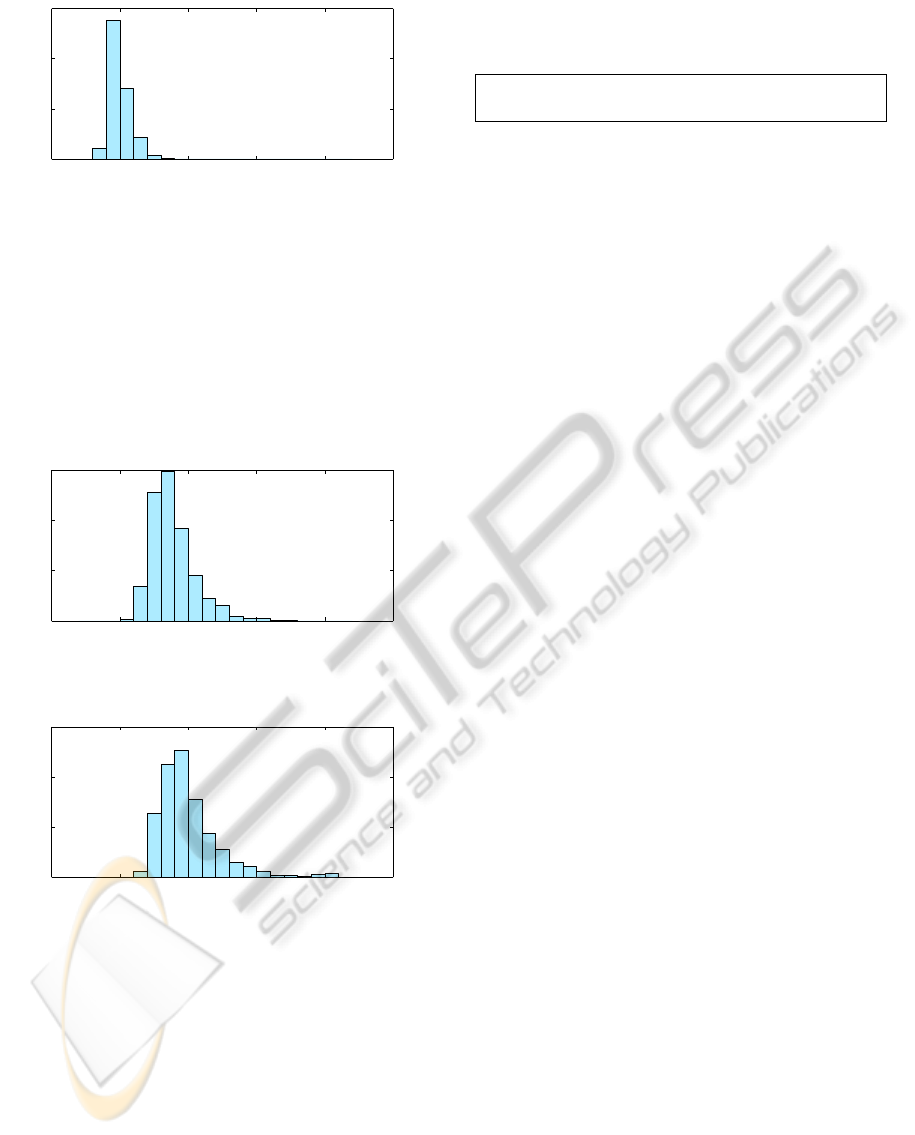
−20 −15 −10 −5 0 5
0
200
400
600
#
log10(res)
Figure 1: Residuals for the (3, 2) solver.
solvers have excellent numerical performance, in par-
ticular the (3, 2) solver, which is expected as it is
just a series of one variable 2nd degree solvers. In
a few instances the (5, 2) solver gives high residuals
or outright fail. This is related to a higher sensitive to
both proximity of degenerate cases and due to a larger
problem size being more prone to cancellation errors.
A total of 1000 experiments per solver were run.
−20 −15 −10 −5 0 5
0
100
200
300
#
log10(res)
Figure 2: Residuals for the (4, 3) solver.
−20 −15 −10 −5 0 5
0
100
200
300
#
log10(res)
Figure 3: Residuals for the (5, 2) solver.
4.2 Real Data
For the experiments with real data 8 microphones
(Shure SV100) were placed on a line along wall in an
office and connected to an audio interface (M-Audio
Fast Track Ultra 8R), which is then connected to a
computer. Relatively distinct sounds were generated
by moving around in the room and clapping. The
8 synchronized channels were recorded at 44.1kHz.
Signal processing was performed by a crude inter-
est point detector on each of the eight signals. In-
terest points were defined as edges between periods
Table 1: Reconstructed microphone array (top) compared
with ground truth (bottom) with origo omitted.
Microphone positions (m)
0.34 0.66 1.00 1.40 1.80 2.14 5.05
0.42 0.69 1.02 1.37 1.77 2.09 4.95
with low energy and periods with high energy. Each
interest point was then matched to the other seven
signals using normalized cross-correlation. Thus ap-
proximately 180 hypothetical matches were found in
the dataset. Among the several error sources in the
setup were reflections in hard surfaces (walls, books,
shelves, computer monitor), receivers not placed per-
fectly collinearly and non-exact estimate of the speed
of sound. A RANSAC procedure using 50 iterations
randomly selecting points and solver (5-2,4-3) saving
the best hypothesis. Scoring here are how many addi-
tional audio signals were consistent within 2dm other
than the 2 or 3 randomly selected. The final result is
obtained using a bundle adjustment (non-linear least
squares) on the found inlier set. Table 1 shows ground
truth and reconstructed coordinates for the points on
the line. Given the error sources and the fact that the
microphones had a diameter of 3 cm the results are
very satisfactory. No ground truth were taken for the
sound sources But the spatial layout (not shown) is
reasonable in regards to the proportions of the office.
5 CONCLUSIONS
In this paper we have studied, modelled and solved
three important minimal cases for structure from
sound assuming that e g the microphones are posi-
tioned on a line. For each of the case we present and
publish efficient and numerically stable solvers. Such
solvers could be used in RANSAC schemes to weed
out the outliers in real data or be integrated in the low-
level audio or radio matching schemes. In the paper
we demonstrate the efficiency and numerical stabil-
ity on simulated data and demonstrate a small system
using low-level feature detection, matching, RANSAC
and bundling, to enable automatic microphone sensor
array calibration using only synchronized audio as in-
put.
REFERENCES
Birchfield, S. T. and Subramanya, A. (2005). Microphone
array position calibration by basis-point classical mul-
tidimensional scaling. IEEE transactions on Speech
and Audio Processing, 13(5).
ICPRAM2013-InternationalConferenceonPatternRecognitionApplicationsandMethods
428

Biswas, R. and Thrun, S. (2004). A passive approach to
sensor network localization. In IROS 2004.
Byr
¨
od, M., Josephson, K., and
˚
Astr
¨
om, K. (2009). Fast and
stable polynomial equation solving and its application
to computer vision. Int. Journal of Computer Vision,
84(3):237–255.
Chen, J. C., Hudson, R. E., and Yao, K. (2002). Maximum
likelihood source localization and unknown sensor lo-
cation estimation for wideband signals in the near-
field. IEEE transactions on Signal Processing, 50.
Elnahrawy, E., Li, X., and Martin, R. (2004). The limits of
localization using signal strength. In SECON-04.
Niculescu, D. and Nath, B. (2001). Ad hoc positioning sys-
tem (aps). In GLOBECOM-01.
Pollefeys, M. and Nister, D. (2008). Direct computa-
tion of sound and microphone locations from time-
difference-of-arrival data. In Proc. of International
Conference on Acoustics, Speech and Signal Process-
ing.
Raykar, V. C., Kozintsev, I. V., and Lienhart, R. (2005). Po-
sition calibration of microphones and loudspeakers in
distributed computing platforms. IEEE transactions
on Speech and Audio Processing, 13(1).
Sallai, J., Balogh, G., Maroti, M., and Ledeczi, A. (2004).
Acoustic ranging in resource-constrained sensor net-
works. In eCOTS-04.
Stew
´
enius, H. (2005). Gr
¨
obner Basis Methods for Mini-
mal Problems in Computer Vision. PhD thesis, Lund
University.
Thrun, S. (2005). Affine structure from sound. In Proceed-
ings of Conference on Neural Information Processing
Systems (NIPS), Cambridge, MA. MIT Press.
Wendeberg, J., Hoflinger, F., Schindelhauer, C., and Reindl,
L. (2011). Anchor-free tdoa self-localization. In In-
door Positioning and Indoor Navigation (IPIN), 2011
International Conference on, pages 1 –10.
MinimalStructureandMotionProblemsforTOAandTDOAMeasurementswithCollinearityConstraints
429
