
A Fluid Limit for the Engset Model
An Application to Retrial Queues
Stylianos Georgiadis
1
, Pascal Moyal
1
, Tam´as B´erczes
2
and J´anos Sztrik
2
1
Laboratoire de Math´ematiques Appliqu´ees de Compi`egne, Universit´e de Technologie de Compi`egne,
Centre de Recherches de Royallieu, BP 20529, 60205, Compi`egne, France
2
Faculty of Informatics, University of Debrecen, Egyetem tr 1, P.O. Box 12, 4010 Debrecen, Hungary
Keywords:
Engset Model, Fluid Limit, Semi-martingale Decomposition, Retrial Queues.
Abstract:
We represent the classical Engset-loss model by the stochastic process counting the number of customers in
the system. A fluid limit for this process is established for all the possible values of the various parameters
of the system, as the number of servers tends to infinity along with the number of sources. Our results are
derived through a semi-martingale decomposition method. A numerical application is provided to illustrate
these results. Then, we represent a finite-source retrial queue considering in addition the number of sources in
orbit. Finally, we extend the fluid limit results to a retrial queueing system, discussing different cases.
1 INTRODUCTION
In many real-life queueing systems of finite capacity,
a customer may find a full system upon arrival. In sev-
eral finite-source models, this requestcan return to the
source and stay there for a randomly distributed time
until it tries again to reach a server. The Engset model
represents a loss queueing system having this input
mechanism for several finite sources producing Pois-
son processes of the same intensity (see, e.g., (Engset,
1918)). We suppose that the system has no buffer,
hence a request is either immediately served or im-
mediately lost, whenever no server is available upon
arrival.
Such a model has been applied to a variety of re-
alistic computer and telecommunication systems and
networks. For exemple, an Engset system is adequate
to represent a radio-mobilenetwork in which the radio
sources emit messages only if no message of the same
source is currently in service. One could think that the
radio sources re-emit the same message as long as the
latter is refused due to the fact that all channels are
busy, and wait to re-issue a new message whenever
the previous message is in treatment.
This model has a wide field of applications, so it
has been studied extensively through analytical and
algorithmic methods as well. However, when the sys-
tem becomes very large, several complexity problems
may appear. The fluid limit technique offers the possi-
bility to approximate the exact values of some charac-
teristics of the system, when one or more parameters
tend to infinity. In our case, the number of servers
tends to infinity along with the number of sources.
Such techniques have been applied fruitfully to many
queueing systems (Robert, 2000; Asmussen, 2003;
Anisimov, 2007; Decreusefond and Moyal, 2012).
Recently, (Feuillet and Robert, 2012) constructed ex-
ponential martingales for the Engset model, allow-
ing to derive asymptotic estimates for several hitting
times of interest. We build on these results to de-
rive the fluid limit of an Engset model having a single
server (Section 3), and then several servers (Section
4). Simulations are presented in Section 5.
In a finite source retrial queue, the messages
which could not reach a serverare sent to the so-called
orbit, from which they are re-emitted on and on, at a
rate that is possibly higher than the original one. It is
then easily seen that the Engset model in nothing but a
particular case of a retrial queueing system for which
the two emission rates are equal. Based on this obser-
vation, in Section 6 we investigate some applications
of our initial result to derive the fluid approximation
of a retrial queue, under various conditions on the sys-
tem parameters.
2 THE ENGSET MODEL
We consider an Engset system with S (S ≥ 1) servers.
There are K (K > S) independent Poisson sources
emitting requests with intensity λ. The service times
315
Georgiadis S., Moyal P., Bérczes T. and Sztrik J..
A Fluid Limit for the Engset Model - An Application to Retrial Queues.
DOI: 10.5220/0004203101170122
In Proceedings of the 2nd International Conference on Operations Research and Enterprise Systems (ICORES-2013), pages 117-122
ISBN: 978-989-8565-40-2
Copyright
c
2013 SCITEPRESS (Science and Technology Publications, Lda.)

of the requests are exponentially distributed of param-
eter µ. Whenever a request finds all servers busy, it is
immediately lost. If not, the request enters service
and the corresponding source remain inactive during
its treatment. As soon as the latter service has been
completed, the source becomes active again, and re-
emit jobs according to a Poisson process of intensity λ
that is independent from the past. In particular, there
is no dependence between the holding times and idle
periods of the sources.
Let X
S
:= (X
S
(t); t ≥ 0) denote the process count-
ing the number of customers in the system (i.e., the
number of busy servers) at current time. X
S
is a
Markov process, whose stationary measure is well-
known and easily derived.
We first examine the Engset queueing model with
a single server, and denote X := X
1
the corresponding
process.
2.1 Semi-martingale Decompositions
Recall (Jacod and Shiryaev, 2003; Decreusefond and
Moyal, 2012) that for a givenFeller Markovprocess Z
of state space E and infinitesimal generator A defined
for all bounded f : E → R by
A f(i) = lim
h→0
1
h
E[ f (X(h)) | X(0) = i]− f(i)
, i∈E,
the process
M
f
: t → f (Z(t)) − f (Z(0)) −
Z
t
0
A f (Z(s)) ds (1)
is a martingale w.r.t. the natural filtration of Z.
For n ≥ 1 fixed, consider an Engset system
M/M/n/n/nK, and add a superscript
n
to all the param-
eters involved. It is easily seen that the infinitesimal
generator A
n
of X
n
reads for all bounded f : R → R
and all i ∈ {0, ..., n},
A
n
f(i) =
=
λ(K −i)( f(i+ 1) − f(i)) + µi( f(i−1) − f(i)),
i ∈{1, ..., n−1};
µn( f(n−1) − f(n)), i = n.
So, taking f as the identity function of {0, ..., n} in
(1), we get
A
n
f(i) = λ(nK −i)1
{i<n}
−iµ,
which leads to the following semi-martingale decom-
position :
X
n
(t) = X
n
(0) −µ
Z
t
0
X
n
(s)ds
+ λ
Z
t
0
(nK −X
n
(s))1
{X
n
(s)<n}
ds+ M
n
(t),
where M
n
is a martingale and X
n
(0) ∈ [0, n].
2.2 The Free Process
The free process describes an Engset model without
limitation in the number of servers, hence an infinite
server queues M/M/∞/∞/nK, having the same input
mechanism. As above, the process Y
n
counting the
number of customers in the system, satisfies the semi-
martingale decomposition
Y
n
(t) = Y
n
(0) −µ
Z
t
0
Y
n
(s)ds
+ λ
Z
t
0
(nK −Y
n
(s)) ds+ P
n
(t)
= Y
n
(0) −(λ + µ)
Z
t
0
Y
n
(s)ds+ λnKt + P
n
(t),
(2)
where P
n
is a martingale.
3 FLUID LIMIT
We are interested in the asymptotic behavior of X
n
(properly rescaled), as the number of servers goes to
infinity together with the number of sources. We ob-
tain hereafter a fluid limit that coincides with that of a
loss Erlang system M/M/n/n, and proceed as in Sec-
tion 6.7 of (Robert, 2000).
We normalize the various processes as follows.
For all t ≥ 0,
¯
X
n
(t) =
X
n
(t)
n
;
¯
Y
n
(t) =
Y
n
(t)
n
.
Assume that the deterministic initial condition satis-
fies
¯
X
n
(0)−→
n→∞
x,
where x ∈ [0, 1] fixed.
We easily check that the semi-martingale equation
(2) is similar to that of an M/M/∞ system of arrival in-
tensity λnK and service durations of parameter λ+ µ.
Whenever
¯
Y
n
(0)−→
n→∞
x, it then follows from Theorem
6.13 of (Robert, 2000) that for all T ≥ 0,
E
sup
0≤t≤T
|
¯
Y
n
(t) −Y
∗
(t) |
−→
n→∞
0, (3)
where, for all t ≥ 0,
Y
∗
(t) = α+ (x−α)e
−(λ+µ)t
, (4)
setting
α =
λK
λ+ µ
.
Let the hitting times
τ
n
:= inf{t ≥ 0;
¯
X
n
(t) = 1}
= inf{t ≥ 0; X
n
(t) = n}
= inf{t ≥ 0; Y
n
(t) = n} (5)
ICORES2013-InternationalConferenceonOperationsResearchandEnterpriseSystems
316

and
τ = inf{t ≥ 0;Y
∗
(t) = 1}. (6)
3.1 Heavy Traffic
First, we examine the case α > 1. Then, we get
τ =
1
λ+ µ
log
α−x
α−1
. (7)
The following lemma follows from Proposition 6 of
(Feuillet and Robert, 2012).
Lemma 1. In heavy traffic, the following convergence
in probability holds for the hitting time (5) :
τ
n
P
−→
n→∞
τ, (8)
where τ is defined by (7).
Theorem 1. For all ε > 0 and all T ≥ 0, we have
P
sup
0≤t≤T
|
¯
X
n
(t) −X
∗
(t) |> ε
−→
n→∞
0,
where, for all t ≥ 0,
X
∗
(t) = 1∧
α+ (x−α)e
−(λ+µ)t
.
Proof. We have
P
sup
0≤t≤T
|
¯
X
n
(t) −X
∗
(t) |> ε
≤ P
sup
0≤t≤T∧τ
n
|
¯
Y
n
(t) −X
∗
(t) |> ε
+ P
inf
τ
n
≤t≤T
¯
X
n
(t) < 1 −
ε
2
+ P
sup
τ
n
≤t≤T
| 1−X
∗
(t) |>
ε
2
. (9)
By the continuity of X
∗
(.), the first and third term on
the r.h.s. of (9) vanish, respectively in view of (3)
and (8). The second term vanishes as it is less than
P(
˜
τ
n
≤t), where
˜
τ
n
is the hitting time of ⌊
nε
2
⌋+ 1 by
Z
n
, the congestion process of an M/M/1 queue with
arrival intensity nµ and service rate λn(K −1). As
nµ < λn(K −1), this queue is stable, so it is a classical
result that
˜
τ
n
is of the order of
λ(K−1)
µ
⌊
nε
2
⌋+1
.
3.2 Light Traffic
Assume now that α < 1.
Theorem 2. In light traffic, for all ε > 0 and all T ≥
0, we have
P
sup
0≤t≤T
|
¯
X
n
(t) −X
∗
(t) |> ε
−→
n→∞
0,
where in that case, for all t ≥ 0,
X
∗
(t) = Y
∗
(t) = α+ (x−α)e
−(λ+µ)t
. (10)
Proof. Notice that
P
sup
0≤t≤T
|
¯
X
n
(t) −X
∗
(t) |
≤ P(τ
n
≤ T) + P
sup
0≤t≤T
|
¯
Y
n
(t) −Y
∗
(t) |> ε
,
and apply (3) together with Markov inequality. The
first term vanishes as τ
n
is asymptotically of the or-
der of (nα
n
)
−1
, as can be shown along the lines of
(Feuillet and Robert, 2012).
3.3 Critical Case
Suppose that α = 1. We reason as above :
Theorem 3. In the critical case, τ
n
is of the order of
log
√
n, hence the same convergence as in Theorem 2
holds true.
4 MULTISERVER ENGSET
MODEL
We now check that the results of Section 3 still hold
true for an Engset queue with S identical servers and
the process X
S
counting the busy servers. We consider
the Engset model M/M/nS/nS/nK. Easily, we obtain
the infinitesimal generator A
n
S
of X
n
S
A
n
S
f(i) = λ(nK −i)1
{i<nS}
−iµ,
and the corresponding semi-martingale decomposi-
tion
X
n
S
(t) = X
n
S
(0) −µ
Z
t
0
X
n
S
(s)ds
+ λ
Z
t
0
(nK −X
n
S
(s))1
{X
n
(s)<nS}
ds+ M
n
S
(t),
where M
n
S
is a martingale and X
n
S
(0) ∈ [0, nS]. The
free process Y
n
S
is given by
Y
n
S
(t) = Y
n
S
(0) −(λ + µ)
Z
t
0
Y
n
S
(s)ds+ λnKt + P
n
S
(t),
where P
n
S
is a martingale. For all t ≥ 0, we consider
the normalized processes
¯
X
n
S
(t) and
¯
Y
n
S
(t) over n and
the limit of the initial condition :
¯
X
n
S
(0)−→
n→∞
x
S
,
where x
S
∈[0, S] fixed. Moreover, we observe that (3)
holds in the case of S servers with Y
∗
S
(t) = Y
∗
(t) and
τ
n
S
= inf{t ≥ 0; Y
n
S
(t) = nS},
τ
S
= inf{t ≥ 0;Y
∗
S
(t) = S}.
Consequently, the hitting time τ
n
S
converges in proba-
bility to
τ
S
=
1
λ+ µ
log
α−x
S
α−S
.
AFluidLimitfortheEngsetModel-AnApplicationtoRetrialQueues
317
Theorem 4. For all ε > 0 and all T ≥ 0, we have
P
sup
0≤t≤T
|
¯
X
n
S
(t) −X
∗
S
(t) |> ε
−→
n→∞
0,
where, for all t ≥ 0, we consider the following cases :
if α > S,
X
∗
S
(t) = S ∧
α+ (x
S
−α)e
−(λ+µ)t
; (11)
if α ≤ S,
X
∗
S
(t) = α+ (x
S
−α)e
−(λ+µ)t
. (12)
As a consequence, the fluid limit for the Engset
system can be derived for any arbitrary, but fixed, val-
ues of the number of sources and servers.
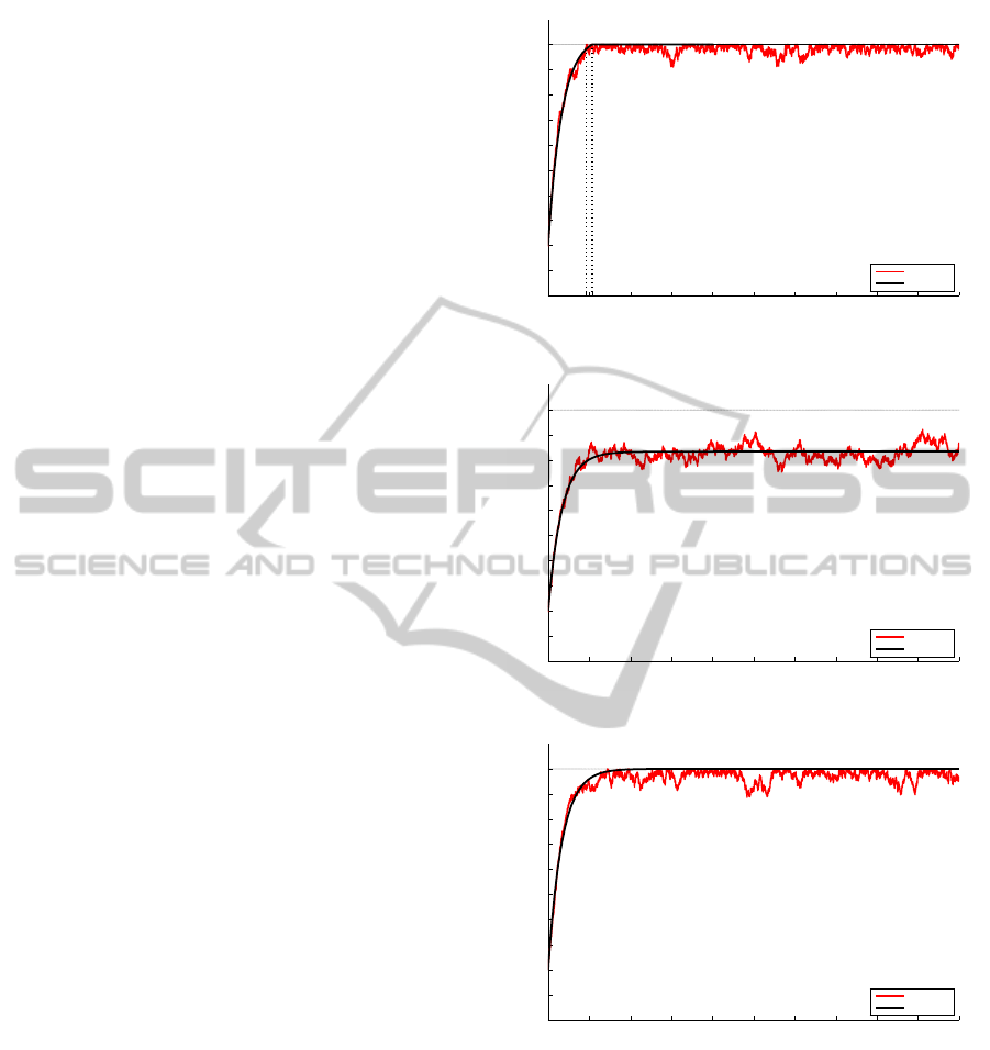
5 NUMERICAL RESULTS
In this section, we present a numerical example for
the multiserver Engset model concerningthe different
cases discussed in Section 4. Consider a M/M/S/S/K
queueing system with parameters S = 500, λ = 0.1
and µ = 0.5. The critical value for the number of
sources is, therefore, K = 3000. Setting various val-
ues for the number of sources, we may obtain the
heavy traffic (α > 500), the light traffic (α < 500) or
the critical case (α = 500). We set the initial value
x
S
= 100 for the busy servers.
In the following figures, we present a realization
of the process X
1
S
of the model described above in the
time interval [0, 50], along with the fluid limit, for the
three cases as given in (11) and (12).
Notice that, in Figure 1, the hitting time of S
servers for the realization (4.6381) is fairly close to
the theoretical value of τ
S
(5.3648).
6 APPLICATION TO SINGLE
SERVER RETRIAL QUEUES
Retrial queues follow the following scenario : when a
customer arriveswith all servers and waiting positions
(if any) being busy, he leaves the service area but after
some randomly distributed time repeats his demand.
For a review of the main results on the topic see (Falin
and Templeton, 1997) and the references therein.
The general queueing system with retrials is de-
scribed more precisely as follows. There are finitely
many identical independent fully available servers at
which requests arrive. Each source can generate a re-
quest with rate λ. If an arriving request finds at least
one server free, it immediately occupies the server
0 5 10 15 20 25 30 35 40 45 50
0
50
100
150
200
250
300
350
400
450
500
Time
Busy Servers
Trajectory
Fluid Limit
Figure 1: Heavy traffic (K > 3000).
0 5 10 15 20 25 30 35 40 45 50
0
50
100
150
200
250
300
350
400
450
500
Time
Busy Servers
Trajectory
Fluid Limit
Figure 2: Light traffic (K < 3000).
0 5 10 15 20 25 30 35 40 45 50
0
50
100
150
200
250
300
350
400
450
500
Time
Busy Servers
Trajectory
Fluid Limit
Figure 3: Critical case (K = 3000).
and leaves it after completion of service. The rate of
service time is denoted by µ. If all servers are busy
at arrival time, then the source goes into the orbit (a
secondary queue of infinite size) and starts the gener-
ation of requests with rate ν until it finds a free server.
After completion of service, the source returns to the
initial state and it can generate a new request, while
the server may serve a new request. All the times in-
volved in the model are assumed to be mutually inde-
pendent of each other.
The presence of the orbit makes the retrial queue-
ICORES2013-InternationalConferenceonOperationsResearchandEnterpriseSystems
318

ing model more flexible than the Engset one, once the
source may generate a message with a different rate
from the rate of the initial state. Actually, an Engset
queue is a special case of the certain finite-source re-
trial system under the condition ν = λ. Because of this
fact, we can apply the results of the previous section
to a retrial queue, and, therefore, investigate different
cases under diverse system parameters.
Consider a single-server retrial queue with finitely
many sources. Let E = {0, 1, . . . , K − 1} and F =
{0, 1}. Let N := (N(t); t ≥ 0) be the number of
sources of in orbit and C := (C(t); t ≥ 0) the num-
ber of busy servers, with state spaces E and F respec-
tively. The system state at time t can be described
by the coupled process A(t) := (N(t),C(t)). The pro-
cess A := (A(t); t ≥ 0) is a continuous-time Markov
process with finite state space E ×F. Since the state
space of the process A is finite, the process is ergodic
with stationary measure
˜
π(·, ·) defined as follows
˜
π(i, j) = lim
t→∞
P(N(t) = i,C(t) = j), i ∈E, j ∈ F.
We consider a sequence of retrial systems with the n-
th one having n servers and nK sources. Let E
n
=
{0, 1, . . . , nK −1} and F
n
= {0, 1, . . . , n}. Let A
n
=
(N
n
,C
n
) be the corresponding process for the n-th
system, with state space E
n
×F
n
.
For all i ∈ E
n
, j ∈ F
n
, we consider the functions
f(i, j) := i and g(i, j) := j. Then, the infinitesimal
operator Q
n
of A
n
applied to f and g reads
Q
n
f(i, j) = −iν1
{j<n}
+ (nK −i−n)λ1
{j=n}
and
Q
n
g(i, j) = [iν+ (nK −i− j)λ − jµ]1
{j<n}
−nµ1
{j=n}
.
which yields the following semi-martingale decom-
positions :
N
n
(t) =N
n
(0) −ν
Z
t
0
N
n
(s)ds
+ (ν−λ)
Z
t
0
N
n
(s)1
{C
n
(s)=n}
ds
+ λn(K −1)
Z
t
0
1
{C
n
(s)=n}
ds+ M
n
1
(t);
hM
n
1
i
t
=ν
Z
t
0
N
n
(s)1
{C
n
(s)<n}
ds
+ λ
Z
t
0
(nK −N
n
(s) −n)1
{C
n
(s)=n}
ds
and
C
n
(t) =C
n
(0) + (ν −λ)
Z
t
0
N
n
(s)1
{C
n
(s)<n}
ds
+ λ
Z
t
0
(nK −C
n
(s))1
{C
n
(s)<n}
ds
−µ
Z
t
0
C
n
(s)ds+ M
n
2
(t);
hM
n
2
i
t
=
Z
t
0
(nK −N
n
(s) −C
n
(s))1
{
C
n
(s)<n}
ds
+
Z
t
0
νN
n
(s)1
{C
n
(s)<n}
ds
+ nµ
Z
t
0
1
{C
n
(s)=n}
ds.
6.1 Law of Large Numbers
We apply the same normalization as in Section 3:
¯
N
n
(t) =
N
n
(t)
n
;
¯
M
1
n
(t) =
M
n
1
(t)
n
;
¯
C
n
(t) =
C
n
(t)
n
;
¯
M
1
n
(t) =
M
n
1
(t)
n
.
Assume that
¯
N
n
(0)−→
n→∞
n
0
;
¯
C
n
(0)−→
n→∞
c
0
,
where n
0
∈ [0, K] and c
0
∈ [0, 1]. Thus, for all t ≥ 0,
we obtain
N
∗
(t) =n
0
+ λ(K −1)
Z
t
0
1
{C
∗
(s)=1}
ds
+ (ν−λ)
Z
t
0
N
∗
(s)1
{C
∗
(s)=1}
ds
−ν
Z
t
0
N
∗
(s)ds; (13)
C
∗
(t) =c
0
+ (ν−λ)
Z
t
0
N
∗
(s)1
{C
∗
(s)<1}
ds
+ λ
Z
t
0
(K −C
∗
(s))1
{C
∗
(s)<1}
ds
−µ
Z
t
0
C
∗
(s)ds. (14)
Theorem 5. The following weak convergence holds :
(
¯
N
n
,
¯
C
n
) ⇒ (N
∗
,C
∗
),
where the deterministic functions N
∗
and C
∗
are the
unique solutions of (13) and (14), respectively.
Proof. We follow the classical steps for proving weak
convergence of processes. The increasing processes
h
¯
M
n
1
i and h
¯
M
n
2
i vanish uniformly on any compact
AFluidLimitfortheEngsetModel-AnApplicationtoRetrialQueues
319

interval as n goes large. Moreover, the Aldous-
Reboledo tightness criterion for semi-martingales
(see, e.g. (Joffe and Mtivier, 1986)) is easily met by
both
¯
N
n
and
¯
C
n
. Thus, the sequence
¯
N
n
(·),
¯
C
n
(·)
is
tight, and any subsequential limit (N
∗
(·), C
∗
(·)) reads
for all t ≥ 0, the equations (13) and (14). The weak
limit is then a solution of this system. The unique-
ness of the latter is easily checked by showing that
the underlying mapping is locally-Lipschitz continu-
ous.
6.2 Discussion
We discuss applications of the latter result in several
cases.
(i) If λ = ν, from (4) and (14), C
∗
coincides with the
fluid limit Y
∗
of Section 3, in the various cases.
Setting, whenever τ is finite (i.e. in the heavy traf-
fic case),
τ
0
= n
0
e
−λτ
,
from the equation (13), we obtain that
N
∗
(t) =n
0
e
−λt
1
{t<τ}
+ (K −1+ [τ
0
−(K −1)]e
−λ(t−τ)
)1
{t≥τ}
.
We check as well the intuitive result that asymp-
totically, the orbit is either full (heavy traffic case)
or empty (light traffic/ critical case).
(ii) Suppose now that Kλ ≤ λ + µ, and fix the initial
condition n
0
= 0. Let
ρ
n
= inf{t ≥ 0; N
n
(t) > 0}.
Up to ρ
n
, no arrival occurs from the orbit, so the
value of ν is irrelevant. It is easily seen that
ρ
n
= τ
n
in distribution,
where τ
n
corresponds to the previous hitting time
for an Engset model. So, from the results of the
previous section in the light traffic and critical
cases, a proof similar to that of Theorem 2 shows
that, for all t ≥ 0,
N
∗
(t) = 0; C
∗
(t) = Y
∗
(t),
where Y
∗
(t) is given in (10).
(iii) All the same, if finally λ < ν and Kλ > ν+ µ, we
show by stochastic comparison of Markov pro-
cesses that
ρ
n
≤
st
τ
n
,
where τ
n
corresponds to a heavily loaded Engset
model of arrival rate λ. So, Theorem 1 entails that
for some 0 < ρ ≤τ, where τ is defined by (6),
C
∗
(t) = 1, for all t ≥ ρ,
i.e. the server is busy all the time after ρ, at the
fluid level.
7 CONCLUSIONS
We have derived the fluid limit of an Engset queueing
system with several servers. After discussing the con-
nection between the Engset queue and retrial queue-
ing models, we present several fluid limit results for
retrial queues. The generalization of the fluid limit
for all possibles values of the parameters λ, µ and ν
of the retrial model, and the numerical confirmation
of their accuracy is a challenging problem that is cur-
rently under investigation.
REFERENCES
Anisimov, V. V. (2007). Switching Processes in Queuing
Models. ISTE-Wiley, Washington.
Asmussen, S. (2003). Applied Probability and Queues.
Spring-Verlag, New York, 2nd edition.
Decreusefond, L. and Moyal, P. (2012). Stochastic Model-
ing and Analysis of Telecom Networks. ISTE-Wiley.
Engset, T. (1918). Die wahrscheinlichkeitsrechnung zur
bestimmung der wahleranzahl in automatischen fern-
sprechamtern. Elektrotech. Zeit., 39(31):304–306.
Falin, G. and Templeton, J. (1997). Retrial Queues. Chap-
man & Hall, London.
Feuillet, M. and Robert, P. (2012). On the transient behav-
ior of Ehrenfest and Engset processes. Advances in
Applied Probability, 44:562–582.
Jacod, J. and Shiryaev, A. (2003). Limit Theorems for
Stochastic Processes. Springer, Berlin, 2nd edition.
Joffe, A. and Mtivier, M. (1986). Weak convergence
of sequences of semimartingales with applications to
multitype branching processes. Advances in Applied
Probability, 18:20–65.
Robert, P. (2000). R´eseaux et Files d’Attente : M´ethodes
Probabilistes. Springer, Paris.
ICORES2013-InternationalConferenceonOperationsResearchandEnterpriseSystems
320
