
Cyclic-type Polling Models with Preparation Times
N. Perel
1
, J. L. Dorsman
2,3
and M. Vlasiou
2,3
1
Department of Statistics and Operations Research, Tel Aviv University, Tel Aviv, Israel
2
Department of Mathematics and Computer Science, Eindhoven University of Technology, Eindhoven, The Netherlands
3
Probability and Stochastic Networks, Centum Wiskunde & Informatica, Amsterdam, The Netherlands
Keywords:
Layered Queuing Networks, Polling Systems, Queuing Theory.
Abstract:
We consider a system consisting of a server serving in sequence a fixed number of stations. At each station
there is an infinite queue of customers that have to undergo a preparation phase before being served. This
model is connected to layered queuing networks, to an extension of polling systems, and surprisingly to
random graphs. We are interested in the waiting time of the server. The waiting time of the server satisfies a
Lindley-type equation of a non-standard form. We give a sufficient condition for the existence of a limiting
waiting time distribution in the general case, and assuming preparation times are exponentially distributed,
we describe in depth the resulting Markov chain. We provide detailed computations for a special case and
extensive numerical results investigating the effect of the system’s parameters to the performance of the server.
1 INTRODUCTION
We study a model that involves one server polling
multiple stations. The server visits N stations in a
cyclic order, serving one customer at a time. At each
station there is an infinite queue of customers that
needs service. Before being served by the server,
a customer must first undergo a preparation phase.
Thus the server, after having finished serving a cus-
tomer at one station, may have to wait for the prepa-
ration phase of the customer at the next station to be
completed. Immediately after the server concludes
his service at some station, another customer from the
infinite queue begins his preparation phase there. Our
goal is to analyse the transient, as well as the long-run,
probabilistic behaviour of this system by quantifying
the waiting time of the server, which is directly con-
nected to the system’s efficiency and throughput.
This model finds wide applications in enterprise
systems, for example when the order of service of
the customers is important. A typical operating strat-
egy in healthcare clinics is to have a specialist rotate
among several stations. The preparation phase rep-
resents the preliminary service a patient typically re-
ceives from an assistant or a nurse. The model, how-
ever, originates from warehousing. It was introduced
in (Park et al., 2003), who consider a storage facility
with bi-directional carousels, where a picker serves
in turns the carousels. The preparation phase repre-
sents the rotation time the carousel needs to bring the
item to the origin, while the service time is the ac-
tual picking time. The authors study the case of two
carousels under specific assumptions. Later on, this
special case for two stations has been further analysed
under general distributional assumptions in (Vlasiou,
2006). The model we consider in this paper gener-
alises this work from two stations to multiple stations.
This extension leads to significant challenges in anal-
ysis, but provides valuable managerial insights. Little
work has been done on multiple-carousel warehouse
systems. Multiple-carousel problems differ intrinsi-
cally from single-carousel problems in a number of
ways. Such systems tend to be more complicated.
The system cannot be viewed as a number of indepen-
dently operating carousels (McGinnis et al., 1986),
since the two separate carousels interact by means of
the picker that is assigned to them. Almost all stud-
ies involving systems with more than two carousels
resort to simulation; see (Litvak and Vlasiou, 2010)
for a complete literature review. This paper offers the
first analytic results for such systems.
This system can also be viewed as an extension
of a 1-limited polling-type system; cf. (Boxma and
Groenendijk, 1988; Eisenberg, 1979; van Vuuren and
Winands, 2007). In general, polling models have at-
tracted a lot of attention in the literature; see e.g.
(Boon et al., 2011; Takagi, 1986; Yechiali, 1993),
and the extensive references therein. Limited polling
212
Perel N., Dorsman J. and Vlasiou M..
Cyclic-type Polling Models with Preparation Times.
DOI: 10.5220/0004206500140023
In Proceedings of the 2nd International Conference on Operations Research and Enterprise Systems (ICORES-2013), pages 14-23
ISBN: 978-989-8565-40-2
Copyright
c
2013 SCITEPRESS (Science and Technology Publications, Lda.)

systems are notoriously difficult to analyse as the
k-limited service discipline does not satisfy the so-
called branching property; see (Resing, 1993). In our
case, we have the added difficulty of an additional
preparation phase before service. Traditional approx-
imation methods seem to be of little help. For exam-
ple, heavy traffic approximations for polling systems
seem to be mainly suitable for the study of charac-
teristics of the customers, as is typical in the polling
literature, rather than the server, as is our case here;
cf. (van der Mei, 2007). Here, we assume that there
are always waiting customers in front of each station.
Therefore, the analysis of the model is parallel to the
study of the server of a polling-type system, in which
each of the queues is overloaded. As such, heavy traf-
fic diffusion approximations cannot be utilised for this
system, since we consider a system that is overloaded,
rather than critically loaded, while fluid approxima-
tions are equally not straightforward due to the addi-
tional preparation phase.
This model is a layered network in which a server,
while executing a service, may request a higher-layer
service and wait for it to be completed. Layered queu-
ing networks occur naturally in all kinds of informa-
tion and e-commerce systems, grid systems, and real-
time systems such as telecom switches; see (Franks
et al., 2009) and references therein for an overview.
Layered queues are characterised by simultaneous or
separate phases where entities are no longer classified
in the traditional roles of “servers” and “customers”,
but may have also a dual role of being either a server
to other entities (of lower layers) or a customer to
higher-layer entities. Think of a peer-to-peer network,
where users are both customers when downloading a
file, but also servers to users who download their files.
For our system, one may view the preparation time
of a customer as a first phase of service. The ser-
vice station (lower layer) acts in this case as a server.
However, the second phase of service (the actual op-
eration) does not necessarily follow immediately. The
service station might have to ‘wait’ for the server to
finish working on other stations. At this stage, the
service stations act as customers waiting to be served
by the higher layer, the server. Thus, we see that
each service station acts both as a ‘server’ (preparing
the customer) and as a ‘customer’ (waiting until the
server completes his tasks in the previous stations).
This model leads to a Lindley-type equation,
which for two stations leads to the equation (in its
steady-state form) as W
D
=
B − A − W
+
. Here, B
denotes the preparation time, A denotes service time
and W is the waiting time of the server. The dif-
ference from the original (Lindley, 1952) equation
is the minus sign in front of W at the right-hand
side of the equation, which in Lindley’s equation is
a plus. Lindley’s equation describes the waiting time
of a customer in a single-server queue. It is one of
the fundamental and best-studied equations in queu-
ing theory. For a detailed study on Lindley’s equa-
tion we refer to (Asmussen, 2003; Cohen, 1982) and
the references therein. The implications of this “mi-
nor” difference in sign are rather far-reaching, since
even for two stations, in the particular case we study
in this paper, Lindley’s equation has a simple solu-
tion, while for our equation it is probably not pos-
sible to derive an explicit expression without making
some additional assumptions. In the applied probabil-
ity literature, there has been considerable interest in
the class of Markov chains described by the recursion
W
n+1
= g(W
n
,X
n
). An important result is the duality
theory by (Asmussen and Sigman, 1996), relating the
steady-state distribution to a ruin probability associ-
ated with a risk process. See also (Borovkov, 1998)
and (Kalashnikov, 2002). However, duality does not
hold in our case, as our function is non-increasing in
its main argument. This fact produces some surpris-
ing results when analysing the equation.
We study the waiting time of the server for this
model. The waiting time satisfies the Lindley-type re-
cursion (2), which surprisingly emerges when study-
ing maximum weight independent sets in sparse ran-
dom graphs. Specifically, consider an n-node sparse
random (potentially regular) graph and let the nodes
of the graph be equipped with nonnegative weights,
independently generated according to some common
distribution. Rather than only the size of the max-
imum independent set, consider also the maximum
weight of an independent set. (Gamarnik et al., 2006)
show that for certain weight distributions, a limiting
result can be proven both for the maximum indepen-
dent set and the maximum weight independent set.
What is crucial in this computation is recursion (2);
cf. (Gamarnik et al., 2006, Eq. (3)). This recursion
provides another surprising link between queuing the-
ory and random graphs.
At a glance, other than the analytical results, the
major insights we gain for this system are summarised
as follows. First, we observe that variability in prepa-
ration times has a greater influence on the system than
that of service times. In the healthcare setting, one
could summarise it as follows: it pays more to have
a reliable nurse than a reliable specialist. See Fig-
ure 1 for an illustration. Second, a small variability of
preparation times actually improves the performance
of the server, in the sense that he waits less frequently;
cf. Figure 2. However, it also decreases the through-
put. Thus, the system’s designer may wish to consider
how to balance these conflicting goals. Next, when
Cyclic-typePollingModelswithPreparationTimes
213

deciding how many stations to assign to a server, the
shape of the distribution plays a role. However, in
general, when preparation times are smaller than ser-
vice times and when the preparation times variability
is low, only few stations per server (about 5 or 6) al-
ready come close to the optimal throughput. The last
insight we gain is of mathematical nature. We ob-
serve that as the number of stations goes to infinity,
the waiting times of the server become uncorrelated.
We additionally provide an analytic lower bound on
the throughput for the general case and an empirical
upper bound. Both bounds are easy to compute, con-
verge exponentially to the true throughput as N goes
to infinity, and are tight in some cases. Thus we get
quick and accurate estimates on the system’s perfor-
mance. For a discussion, see Section 4.
The rest of the paper is organised as follows: the
general model is presented in the next section where
we also give a sufficient condition for the existence
of a limiting waiting-time distribution. Under the as-
sumption that preparation times are exponential, we
study the transient behaviour of the waiting time in
Section 3 and provide the transition matrix of the un-
derlying Markov chain. We conclude in Section 4
with insights to the effect of all parameters to the sys-
tem’s performance and gives the main conclusions.
2 GENERAL MODEL
We assume that there are N ≥ 2 identical stations op-
erated by a single server. The system operates as
follows. Before being served by the server, a cus-
tomer must first undergo a preparation phase (not in-
volving the server). Thus the server, after having fin-
ished serving a customer at one station, may have to
wait for the preparation phase of the customer at the
next station to be completed. Immediately after the
server concludes his service at some station, another
customer from the queue begins his preparation phase
there while the server moves to the next station. We
are interested in the waiting time of the server. Let B
n
denote the preparation time for the n-th customer and
let A
n
be the time the server spends on this customer.
Then the waiting times W
n
of the server satisfy
W
n+1
=
B
n+1
−
n
∑
i=n−N+2
A
i
−
n
∑
i=n−N+2
W
i
+
. (1)
We assume that each sequence {A
n
}
n≥1
and {B
n
}
n≥1
is comprised of independent, identically distributed
(i.i.d) nonnegative random variables with finite
means, and the sequences are mutually independent.
Moreover, for all n ≥ 1, A
n
(B
n
) have a general distri-
bution function F
A
(F
B
), density function f
A
( f
B
) and
Laplace-Stieltjes Transform (LST) α(s) = E
e
−sA
(β(s) = E
e
−sB
). Eq. (1) can be written as
W
n+1
=
X
n+1
−
n
∑
i=n−N+2
W
i
+
, (2)
where X
n+1
= B
n+1
−
∑
n
i=n−N+2
A
i
. Note that {X
n
}
are identically distributed for n ≥ N according to a
random variable X , but are not independent. They
are only independent with a N − 1-lag. For exam-
ple, {X
N
, X
2N−1
, X
3N−2
, X
4N−3
,...} are indepen-
dent. We also define R
j
n
to be the residual prepa-
ration time in station (n + j) mod N at the moment
the server is available for the n-th time, n ≥ 1, j =
1,...,N − 2. Clearly, R
N−1
n
= B
n+N−1
and R
N
n
= W
n
.
Note that we distinguish between stations and visits.
Since the server attends the stations in a cyclic or-
der, starting the n-th visit is equivalent to visiting sta-
tion j = n mod N for the d
n
N
e-th time. The process
(W
n
,R
1
n
,R
2
n
,...,R
N−2
n
) is a Markov chain, of which
the evolution is given by
W
n+1
=
R
1
n
−W
n
− A
n
+
,
R
j
n+1
=
R
j+1
n
−W
n
− A
n
+
for j = 1,2,...,N − 2.
Last, we assume that P(X ≤ 0) > 0, omitting the sub-
script when we consider a generic random variable.
2.1 Existence of a Limiting Waiting
Time Distribution
Recall that X
n+1
= B
n+1
−
∑
n
i=n−N+2
A
i
, so that
X
N
,X
N+1
,... are identically distributed. Note that the
stochastic process {W
n
} is a (possibly delayed) re-
generative process with regeneration times {n : W
n
=
W
n+1
= ... = W
n+N−2
= 0}. Moreover, note that this
process is aperiodic. Let j be any regeneration time
after t = N − 1. Furthermore, let τ = inf{n : n >
0,W
j
= W
j+1
= . . . = W
j+N−2
= W
j+n
= W
j+n+1
=
... = W
j+n+N−2
= 0}, so that τ can be interpreted as
the time between two regeneration moments. In the
Appendix, we show that the mean cycle length E[τ]
is finite, which implies by standard theory on regen-
erative processes that the limiting distribution of the
waiting time exists and the waiting-time process con-
verges to it (see e.g. (Asmussen, 2003, Cor. VI.1.5
and Thm. VII.3.6)).
3 TRANSIENT ANALYSIS
For the sequel, we assume that preparation times are
exponentially distributed with rate µ. Note that the
analysis can extend to phase-type preparation times,
ICORES2013-InternationalConferenceonOperationsResearchandEnterpriseSystems
214

but at the cost of more cumbersome expressions. Fur-
thermore, little insight is added by such an extension.
We first show that the waiting time (has an atom
at zero and), provided that it is positive, is also ex-
ponentially distributed with rate µ. We then com-
pute the atom at zero by computing the transition
matrix of the underlying Markov chain. We show
that the matrix has a nice structure that can be ex-
ploited for numerical computations. Particularly for
three stations, we provide further analytic results.
We compute the steady-state distribution, and give
closed-form expressions for the covariance between
two waiting times and for the mean time between
two zero waiting times, both for the transient and the
steady-state cases.
3.1 The Behaviour of W
n+1
We show that P(W
n+1
> x | W
n+1
> 0) = e
−µx
, for all
n ≥ 0. We prove this claim for n ≥ N − 1 (for 1 ≤ n ≤
N −2 it is done in a similar way). In order to calculate
P(W
n+1
> x), we first calculate it conditioned on the
last N − 1 waiting times. We get, for all n ≥ N − 1,
P(W
n+1
> x|W
n
= w
n
,...,W
n−N+2
= w
n−N+2
)
= P(B
n+1
>
n
∑
i=n−N+2
A
i
+
n
∑
i=n−N+2
w
i
+ x)
=
Z
∞
0
···
Z
∞
0
e
−µ(
∑
n
i=n−N+2
(y
i
+w
i
)+x)
dF
A
n−N+2
(y
n−N+2
)...dF
A
n
(y
n
)
= (α(µ))
N−1
exp{−µ(
N
∑
i=n−N+2
w
i
+ x)}, (3)
where we defined α(µ) = E
e
−µA
. Thus, (3) implies
that
P(W
n+1
> x |
n
∑
i=n−N+2
W
i
= 0) = (α(µ))
N−1
e
−µx
.
From (3) we also get that
P(W
n+1
> x|W
n+1
> 0,W
n
= w
n
,...,
W
n−N+2
= w
n−N+2
)
=
P(W
n+1
> x | W
n
= w
n
,...,W
n−N+2
= w
n−N+2
)
P(W
n+1
> 0 | W
n
= w
n
,...,W
n−N+2
= w
n−N+2
)
=
(α(µ))
N−1
exp{−µ(
∑
n
i=n−N+2
w
i
+ x)}
(α(µ))
N−1
exp{−µ(
∑
n
i=n−N+2
w
i
)}
= e
−µx
,
meaning that, given W
n+1
> 0, W
n+1
is not
affected by the previous N − 1 waiting times
W
n
,W
n−1
,...,W
n−N+2
. A direct conclusion is that
P(W
n+1
> x|W
n+1
> 0) = e
−µx
and thus, for x > 0,
P(W
n+1
> x) = P(W
n+1
> x | W
n+1
> 0)P(W
n+1
> 0)
+ P(W
n+1
> x | W
n+1
= 0)P(W
n+1
= 0)
= e
−µx
P(W
n+1
> 0). (4)
That is, the distribution of W
n
is a mixture of a mass at
zero and the exponential distribution with rate µ. The
same argument can be applied in a similar manner for
W , the limit of W
n
as n → ∞. That is, P(W > x) =
e
−µx
P(W > 0). We now calculate P(W
n+1
> 0) for all
n, and P(W > 0). In order to do that, we will define
a Markov chain and calculate its one-step transition
probability matrix. A detailed analysis is presented in
the next section.
3.1.1 Construction of a Markov Chain
Recall that the process (W
n
,R
1
n
,R
2
n
,...,R
N−2
n
) is a
Markov chain and define the auxiliary 0-1 random
variables F
n
= I(W
n
> 0) and G
j
n
= I(R
j
n
> 0), j =
1,...,N − 2. That is, F
n
= 0 if, at the moment the
server starts his n-th visit to a station, the customer
there completed his preparation process, so that the
server does not have to wait. Otherwise, F
n
= 1. In
the same way, G
j
n
= 0 if, at the moment the server
starts his n-th visit to a station, the customer at station
(n + j) mod N has completed the preparation process,
and G
j
n
= 1 otherwise.
Due to the memoryless property of the prepara-
tion times, the process (F
n
,G
1
n
,...,G
N−2
n
) is a Markov
chain on {0,1}
N−1
. Thus, the state space consists of
2
N−1
states, where each state describes the residual
preparation time in each station (positive or zero) at
the moment the server enters a station for his overall
n-th visit. The only station that does not appear in this
description is the station the server has just left, since
the residual preparation time there is always B (or, in
other words, G
N−1
n
= 1 for all n). Let P be the one-
step transition probability matrix of the Markov chain
(F
n
,G
1
n
,...,G
N−2
n
), where the states are lexicograph-
ically ordered, so that the first state is (0,0,...,0,0),
the second one is (0,0,...,0,1), and so on, where the
last state is (1, 1, . . . , 1, 1). For a state i ∈ {0,1}
N−1
we denote its coordinates by (i
0
,...,i
N−2
). Below,
we describe how to construct the matrix P.
Theorem 1. The transition matrix P is described as
follows. For a state i ∈ {0,1}
N−1
, define T (i) = {r :
p
i,r
> 0} and k =
∑
N−2
r=0
i
r
. For j ∈ T (i) also define
m =
∑
N−2
r=0
j
r
and d = k − m. If F
n
= 0, then
P
i, j
=
(
α(mµ) if d = −1,
∑
d+1
l=0
d+1
l
(−1)
l
α((m + l)µ) if d > −1.
For F
n
= 1, we have
P
i, j
=
(
α(mµ)
m+1
if d = 0,
∑
d
l=0
d
l
(−1)
l
α((m+l)µ)
m+l+1
if d > 0.
For all other values of d, P
i, j
= 0.
Cyclic-typePollingModelswithPreparationTimes
215

Proof. For each state i ∈ {0,1}
N−1
, we derive the
possible target states, namely T (i), as follows: move
all 0’s (except the first one if F
n
= 0) one po-
sition to the left and take all possible combina-
tions for the other positions. This sums up to ei-
ther 2
k
or 2
k+1
possible states, depending on the
value of F
n
. For example, for N = 4, assume
the chain is in state (0,1,0), then T [(0, 1, 0)] =
{(0,0,0),(0,0,1),(1,0,0),(1,0,1)}.
Assume F
n
= 0, meaning that at the current state,
the server starts serving immediately upon entering
the station.
• If d = −1, then all stations that had a positive resid-
ual preparation time in state i, will still have a pos-
itive residual preparation time in state j. In addi-
tion, the preparation time in the station the server
has just left did not end as well. As d = −1 implies
m = k + 1, this transition occurs when during the
service time A, k + 1 = m independent exponential
preparation times with rate µ were not completed.
Therefore,
P
i, j
=
Z
∞
0
e
−mµy
dF
A
(y) = α(mµ).
• When d > −1, exactly k + 1 − m = d + 1 prepara-
tion times have ended during a service time A, and
the other m did not. Thus,
P
i, j
=
Z
∞
y=0
(1 − e
−µy
)
d+1
e
−mµy
dF
A
(y)
=
d+1
∑
l=0
d + 1
l
(−1)
l
α((m + l)µ).
We now consider the case where F
n
= 1, imply-
ing that the preparation in the station the server had
just entered did not finish, and thus an exponential
preparation time B remains. Note that when F
n
= 1,
d = k − m is nonnegative.
• The case d = 0 means that (i) all stations with a pos-
itive residual preparation time in state i, will still
have a positive residual preparation time in state
j, and (ii) the preparation time in the station that
the server has just left also did not end. Namely,
this transition occurs when during the preparation
time B and service time A, k = m independent expo-
nential preparation times with rate µ were not com-
pleted. Therefore,
P
i, j
=
ZZ
R
2
+
e
−mµ(x+y)
µe
−µx
dxdF
A
(y) =
α(mµ)
m + 1
.
• When d > 0, exactly k − m = d out of k prepara-
tions have been completed during the time A + B,
implying that
P
i, j
=
Z
∞
y=0
Z
∞
x=0
(1 − e
−µ(x+y)
)
k−m
e
−mµ(x+y)
µe
−µx
dxdF
A
(y)
=
d
∑
l=0
d
l
(−1)
l
α((m + l)µ)
m + l + 1
.
Once the matrix P is computed, we can find the
distribution of W
n
for all n ≥ 1, which is given in (4).
Therefore, we need P(W
n
> 0).
Let π
n
denote the distribution vector on all the
2
N−1
possible states at the moment the server starts
his n-th visit. Recall that the states are lexicographi-
cally ordered. We may assume that the Markov chain
starts at time 1 from has an initial distribution vec-
tor π
1
= (0,0,...,0,0,1), meaning that at the mo-
ment the server enters the first station, in all sta-
tions the preparation has not been completed yet, and
therefore the Markov chain at that moment is in state
(1,1,...,1,1). Now, P(W
n
> 0) is the sum of the last
2
N−2
elements of the vector π
1
P
n−1
. Furthermore,
we can also find the distribution of W (which is the
limiting distribution of W
n
), by solving the equation
πP = π, and by summing the last 2
N−2
elements of π
(all the states that start with 1), we get P(W > 0).
Next we present a detailed analysis for the case
with N = 3 stations. We again consider exponentially
distributed preparation times, although the analysis
can evidently extend to phase-type distributions.
3.2 Analysis for N = 3 Stations
For N = 3, the evolution of the Markov process
(W
n
,R
n
) is given by
W
n+1
= (R
n
−W
n
−A
n
)
+
, R
n+1
= (B
n+2
−W
n
−A
n
)
+
,
where W
n
is the waiting time of the server at his n-th
entrance to a station, and R
n
is the residual prepara-
tion time in the following station. Clearly, the residual
preparation time in the station that was just left by the
server is B. We assume that the preparation time in
each station is exponentially distributed with param-
eter µ. We calculate the limiting distribution (W,R)
of the Markov chain and the (transient) distribution
of W
n
. We also derive the covariance Cov[W
n
,W
n+k
,]
and the distribution function of the number of vis-
its between two successive zero waiting times of the
server. Observe that these are not necessarily two re-
generative points. We first need to derive the transi-
tion probabilities of the Markov chain.
As described in Section 3.1.1, there are only four
(2
3−1
) relevant states in the corresponding Markov
chain. Define π = (π
(0,0)
,π
(0,1)
,π
(1,0)
,π
(1,1)
) to be
ICORES2013-InternationalConferenceonOperationsResearchandEnterpriseSystems
216

the stationary probabilities vector of the states {(0,0),
(0,1), (1,0), (1,1)}. Let P
(i, j),(k,l)
be the one-step tran-
sition probabilities, i.e.
P
(i, j),(k,l)
= P(F
n+1
= k,G
n+1
= l|F
n
= i, G
n
= j),
for i, j,k,l = 0, 1. By Theorem 1 we get that P is given
by
P =
1 − α(µ) α(µ) 0 0
1 − 2α(µ) +α(2µ) α(µ) − α(2µ) α(µ) − α(2µ) α(2µ)
1 −
1
2
α(µ)
1
2
α(µ) 0 0
1 − α(µ) +
1
3
α(2µ)
1
2
α(µ) −
1
3
α(2µ)
1
2
α(µ) −
1
3
α(2µ)
1
3
α(2µ)
Thus, we obtain the limiting distribution
π
(0,0)
=
12−6α
2
(µ)−12α(µ)+4α(µ)α(2µ)+α
2
(µ)α(2µ)+8α(2µ)
12+6α
2
(µ)+α
2
(µ)α(2µ)+8α(2µ)
,
π
(0,1)
=
4α(µ)(3−α(2µ))
12+6α
2
(µ)+α
2
(µ)α(2µ)+8α(2µ)
,
π
(1,0)
=
2α(µ)(α(µ)α(2µ)+6α(µ)−6α(2µ))
12+6α
2
(µ)+α
2
(µ)α(2µ)+8α(2µ)
,
π
(1,1)
=
12α(µ)α(2µ)
12+6α
2
(µ)+α
2
(µ)α(2µ)+8α(2µ)
.
To obtain the transient distribution and the covari-
ance function, let π
1
= (0,0,0,1) be the initial vector
of the Markov chain (F
n
,G
n
). Then, for all x ≥ 0
P(W
n
> x) = e
−µx
P
(n−1)
[4,3] + P
(n−1)
[4,4]
,
with P[i, j] the element in row i and column j. Now,
Cov[W
n
,W
n+k
] = E[W
n
W
n+k
] − E[W
n
]E[W
n+k
].
Since W
n
|
W
n
>0
∼ exp(µ), we have for all k ≥ 0,
E[W
n+k
] = E[W
n+k
|W
n+k
> 0]P(W
n+k
> 0)
=
1
µ
P(W
n+k
> 0).
To calculate E[W
n
W
n+k
], we note that
E[W
n
W
n+k
] = E[W
n
W
n+k
|W
n
> 0,W
n+k
> 0]
P(W
n
> 0,W
n+k
> 0),
where
E[W
n
W
n+k
|W
n
> 0,W
n+k
> 0]
=
Z
∞
w=0
wE[W
n+k
|W
n+k
> 0,W
n
> w]µe
−µw
dw
=
Z
∞
w=0
w
1
µ
µe
−µw
dw =
1
µ
2
,
and
P(W
n+k
> 0,W
n
> 0)
= P(W
n+k
> 0|W
n
> 0)P(W
n
> 0)
= P(W
n
> 0)(P(W
n+k
> 0|W
n
> 0, R
n
= 0)
P(R
n
= 0|W
n
> 0)
+ P(W
n+k
> 0|W
n
> 0, R
n
> 0)P(R
n
> 0|W
n
> 0))
=
P
(k)
[3,3] + P
(k)
[3,4]
P
(n−1)
[4,3]
+
P
(k)
[4,3] + P
(k)
[4,4]
P
(n−1)
[4,4].
Therefore,
E[W
n
W
n+k
] =
1
µ
2
P
(k)
[3,3]+ P
(k)
[3,4]
P
(n−1)
[4,3]
+
P
(k)
[4,3]+ P
(k)
[4,4]
P
(n−1)
[4,4]
. (5)
Finally,
Cov[W
n
,W
n+k
] = E[W
n
W
n+k
]
−
1
µ
2
P(W
n
> 0)P(W
n+k
> 0),
with E[W
n
W
n+k
] given in (5).
Last, we compute the distribution and expectation
of visits between two consecutive zero waiting times.
Suppose that W
n
= 0 and define for all n ≥ 1 the ran-
dom variable C
n
:=C
|W
n
=0
, describing the length from
the moment that W
n
= 0 until the next time that the
server’s waiting time is zero. In other words,
C
n
= inf{k : W
n+k
= 0 | W
n
= 0}.
The results are summarised in the following theorem.
Theorem 2. The distribution of C
n
is given by
P(C
n
= 1) = 1 −
P
(n−1)
[4,2]
P
(n−1)
[4,1]+ P
(n−1)
[4,2]
α(µ), (6)
P(C
n
= 2) =
P
(n−1)
[4,2]
P
(n−1)
[4,1]+ P
(n−1)
[4,2]
α(µ)
1 −
1
2
α(2µ)
,
P(C
n
= k) =
P
(n−1)
[4,2]
P
(n−1)
[4,1]+ P
(n−1)
[4,2]
α(µ)
1
2
α(2µ)
1
3
α(2µ)
k−3
1 −
1
3
α(2µ)
, k ≥ 3.
Moreover,
E[C
n
] = 1 +
P
(n−1)
[4,2]
P
(n−1)
[4,1]+ P
(n−1)
[4,2]
α(µ)
6 + α(2µ)
6 − 2α(2µ)
. (7)
Proof. For k = 1, we have that
P(C
n
= 1) = P(W
n+1
= 0|W
n
= 0)·
= P(W
n+1
= 0|W
n
= 0,R
n
= 0)P(R
n
= 0|W
n
= 0)
+ P(W
n+1
= 0|W
n
= 0,R
n
> 0)P(R
n
> 0|W
n
= 0)
= (P[1,1]+ P[1, 2]) ·
P
(n−1)
[4,1]
P(W
n
= 0)
+ (P[2,1] + P[2,2]) ·
P
(n−1)
[4,2]
P(W
n
= 0)
=
P
(n−1)
[4,1]
P(W
n
= 0)
+ (1 − α(µ)) ·
P
(n−1)
[4,2]
P(W
n
= 0)
= 1 − α(µ)
P
(n−1)
[4,2]
P
(n−1)
[4,1]+ P
(n−1)
[4,2]
.
Cyclic-typePollingModelswithPreparationTimes
217

The results for
P(C
n
= i)
= P(W
n+i
= 0,W
n+i−1
> 0, . . . ,W
n+1
> 0|W
n
= 0)
with i > 1, follow by expanding this expression into
P(W
n+1
> 0|W
n
= 0) as well as probabilities of the
form P(W
j+2
> 0|W
j+1
> 0,W
j
= 0) and P(W
j+2
>
0|W
j+1
> 0,W
j
> 0). Similar to the derivations above,
these probabilities can be computed by using the
Markov chain formulation of the previous section.
The proof of (7) is straightforward.
4 INSIGHTS
In the previous sections, we gave closed-form expres-
sions for exponentially distributed preparation times.
Here, we obtain general insights into the behaviour
of the model by simulation on a larger range of pa-
rameter settings. We vary, among other, the num-
ber of stations and the distributions of the preparation
and service times. We focus on the effect of the first
two moments of preparation and service times to the
throughput. For their distributions, we choose phase-
type distributions based on two-moment-fit approxi-
mations commonly used in literature, see e.g. (Tijms,
1994, p. 358–360). We discuss several interesting
conclusions based on the simulation results.
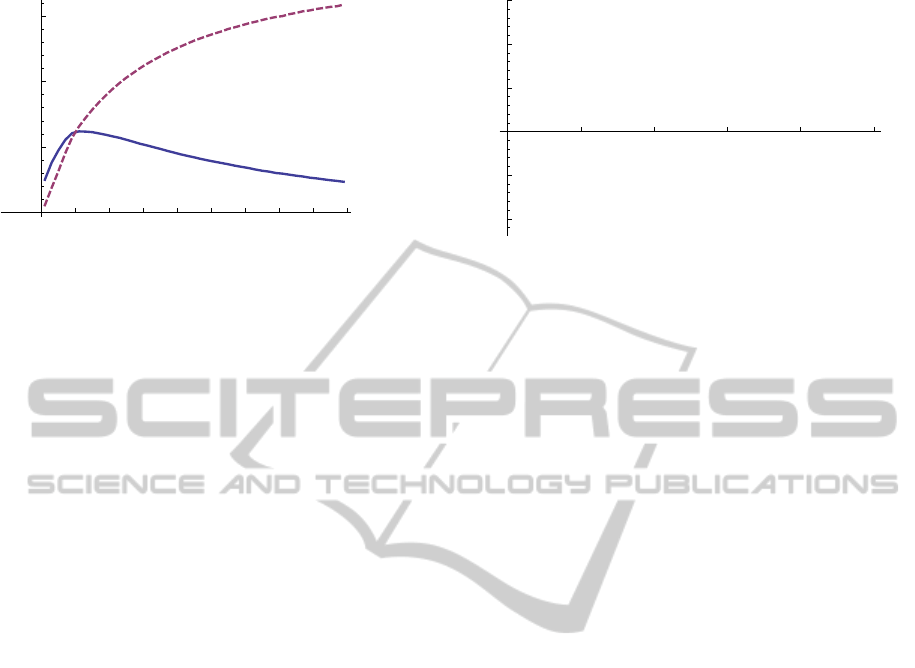
Variability of Preparation and Service Times.
When controlling the system, the variability of the
preparation times seems to play a larger role than
the variability of the service time. This is because
the server’s waiting-time process is much more sen-
sitive to the former than to the latter. See e.g. Fig-
ure 1, where the throughput θ is plotted versus the
number of queues N. We observe the throughput
for various variability settings for both time compo-
nents. We fix the means at E[A] = E[B] = 1, and
consider the exponential distribution, i.e. E[A
2
] =
E[B
2
] = 2 (solid curve), and two different phase-
type distributions with highly variable service times
only, i.e. E[A
2
] = 10, E[B
2
] = 2 (dotted curve) and
highly variable preparation times only, i.e. E[A
2
] =
2,E[B
2
] = 10 (dashed curve). Although the variabil-
ity of preparation times and service times are var-
ied in similar ways, the dotted curve nears the solid
curve as N grows larger much faster than the dashed
curve. Therefore, predictability of the preparation
times seems to be much more important than that of
the service times. This is to be expected; when we ob-
serve (1) we see that as the number of stations tends
to infinity, the squared coefficient of variation of the
sum of service times at the right-hand side of (1) goes
æ
æ
æ
æ
æ
æ
æ
æ
æ
æ
æ
æ
æ
æ
à
à
à
à
à
à
à
à
à
à
à
à
à
à
ì
ì
ì
ì
ì
ì
ì
ì
ì
ì
ì
ì
ì
ì
2
3
4
5
6
7
8
9
10
11
12
13
14
15
N
0.6
0.7
0.8
0.9
1.0
Θ
Figure 1: Throughput vs. the number of stations for
standard-exponential preparation and service times (solid),
highly variable service times (dotted) and highly variable
preparation times (dashed).
to zero, and thus the effect of the sum of the service
times is minimal.
In other words, it is more important that one has
a reliable assistant than a reliable server, in partic-
ular for large systems. In the carousel setting, this
is more or less guaranteed; although the prepara-
tion times (i.e. rotation times) depend on the pick-
ing strategy followed, they are bounded by the length
of the carousel and as such exhibit small variabil-
ity. Whether the picker is robotic (small variability)
or human, does influence the system, but not as dra-
matically as the preparation times do. The influence
of variable service times decreases very fast as the
number of stations increases, even for highly variable
service times. The influence of variable preparation
times decreases too but so slowly that it converges to
the benchmark case only at infinity. It is natural to ex-
pect that as N tends to infinity preparation times be-
come less important. One expects that the preparation
will almost surely have expired after serving a very
large number of stations and that the total throughput
will simply equal the rate of service.
This statement is reinforced by Figure 2, where
the mean time between two zero waiting times is plot-
ted versus the second moment of the preparation time
B (solid curve) or that of the service time A (dashed
curve). It is assumed that N = 4 and E[A] = E[B] = 1
throughout for both of these lines. For the first curve,
the service times A are taken to be exponentially dis-
tributed, while for the second, the preparation times
B are taken to be exponentially distributed. From
Figure 2, it is apparent that the mean time between
two zero waiting times increases (i.e. the frequency
of zero waiting times decreases) as the service times
becomes more variable. However, mostly the oppo-
site is observed for the preparation times. Although
the expected waiting time increases in the variabil-
ICORES2013-InternationalConferenceonOperationsResearchandEnterpriseSystems
218
2
3
4
5
6
7
8
9
10
E@A
2
Dor E@B
2
D
1.10
1.15
1.20
E@CD
Figure 2: Mean time between two zero waiting times vs.
E[B
2
] (solid) and E[A
2
] (dashed).
ity of the preparation times by Figure 1, apparently
the mean time between two zero waiting times now
decreases anomalously. From this, we conclude that
the server’s waiting time process behaves more and
more erratically as the variability of the preparation
times increases and seems to be more resistent against
highly variable service times. Again, this effect may
be explained by the nature of the waiting time (see
(1)), which is expressed in terms of one preparation
time, but a sum of service times. The squared coeffi-
cient of variation of the sum goes to zero.
In summary, we can say that variability of prepa-
ration times, as long as it is small, improves the per-
formance of the server, in the sense that he waits
less frequently, while variability of service times al-
ways improves the performance of the server in the
same sense. However, both scenarios decrease the
throughput of the system – although waiting times
occur less frequently under some variability, when
they occur they tend to be longer, thus decreasing
the total throughput. Simulation results show about
a 10% decrease in throughput under common scenar-
ios when ranging the preparation time variability (i.e.
the worst case) from a deterministic to an exponential.
Nonetheless, in some service systems this may be an
advantage, as it gives the opportunity to perform an
additional task (e.g. administration).
Correlations. In general, this system has an inter-
esting correlation structure. In Figure 3 we plot the
correlation between two waiting times of lag k against
the lag for exponential preparation and service times
with rates 1 and 10 respectively. As we see in Fig-
ure 3, correlations exhibit a periodic structure, which
is natural as it corresponds to a return to the first sta-
tion. Moreover, as time goes to infinity, the waiting
times become uncorrelated, which is again a natural
conclusion, as the process is ergodic. As shown in
Section 2.1, there exists a unique limiting distribution
and the system converges to it, thus as time (or the
æ
æ
æ
æ
æ
æ
æ
æ
æ
æ
æ
æ
æ
æ
æ
æ
æ
æ
æ
æ
æ
æ
æ
æ
æ
5
10
15
20
25
k
-0.10
-0.05
0.05
0.10
0.15
Corr@W
n
, W
n+k
D
Figure 3: Correlations exhibit periodicity.
number of stations for that matter) goes to infinity, the
system converges to steady-state regardless of the ini-
tial state. Thus, the correlation between waiting times
goes to zero because the system loses its memory due
to ergodicity. Although the convergence to zero corre-
lations is expected, the way this happens is intriguing.
One may expect some form of periodicity, but it is not
clear why the first cycle looks different than the rest
or why correlations should be forming alternatingly
convex and concave loops after the first cycle.
Number of Stations to be Assigned to a Server.
One of the important management decisions to be
made is the number of stations to be assigned to a
server. Think of the warehouse example given ear-
lier. The more carousels assigned to the picker, the
better his utilisation. However, the utilisation of each
carousel decreases. We wish to understand this in-
terplay. An important measure to be taken into ac-
count is the throughput of the system. Note that the
throughput is linearly related to the fraction of time
the server is operating, since service is completed at
rate E[B]
−1
whenever the server is not forced to wait.
The number of stations to be assigned to a server in
order to reach near-optimal throughput depends very
much on the distributions of the preparation time B
and the service time A. This effect is observed in Fig-
ure 1, where we see that for highly variable prepara-
tion times (dashed line), the throughput increases for
every additional station assigned to the server. Evi-
dently, it will converge to the rate of service, but this
convergence is very slow. On the other hand, variabil-
ity in the service times influences the system, but the
convergence follows more or less the pattern of the
exponential case.
When all distributions are exponential, it is evi-
dent that the only quantity that matters in the determi-
nation of the throughput is r = E[A]/E[B]. In order to
determine the optimal number of stations to assign to
a server, we plot in Figure 4 the throughput θ versus
the number of stations N for three cases of r, namely
Cyclic-typePollingModelswithPreparationTimes
219

æ
æ
æ
æ
æ
æ
æ
æ
æ
æ
æ
æ
æ
æ
æ
æ
æ
æ
æ
æ
æ
æ
æ
æ
æ
æ
æ
æ
æ
æ
æ
æ
æ
æ
æ
æ
æ
æ
æ
æ
æ
æ
2
4
6
8
10
12
14
N
0.4
0.5
0.6
0.7
0.8
0.9
1.0
Θ
Figure 4: Throughput vs. the number of stations for small
(dashed), moderate (solid), and large preparation times
(dotted).
for r = 2 (top curve), r = 1 (solid curve), and r = 0.5
(dotted curve). In all three cases, the underlying dis-
tributions are exponential. What we observe is that
when r ≥ 1, i.e. the top two curves, the throughput
converges fast, and little benefit is added by assign-
ing one more station to the server. This is to be ex-
pected, as in this case the mean service time is not
smaller than the mean preparation time, and so the
server rarely has to wait. In other words, he works
at almost full capacity, and thus convergence to the
maximum service rate (equal to 1 in all scenarios), is
fast. However, when r < 1, the convergence is very
slow. We conclude that the shape of the distribution
plays a role, but in general for r > 1 and low vari-
ability in preparation times will, only few stations per
server (say about 5 or 6) are needed to already come
close to the maximum throughput.
A Rough Estimate. In Figure 4 we also plot a
rough first-order upper bound and an analytic lower
bound of the throughput that we derive as follows.
The throughput θ of the system is equal to the number
of customers N served per cycle over the cycle length,
which is N(E[W ] + E[A]). Thus,
θ = (E[W ] + E[A])
−1
.
A first-order approximation of θ can be produced by
estimating E[W ] in the denominator with the mean
residual preparation time multiplied with a rough es-
timate that the server has to wait, i.e. P(B > A
1
+···+
A
N−1
). Then, for exponential preparation times B,
e
θ
N
=
1
α
N−1
(µ)
µ
+ E[A]
.
We observe that this expression is a lower bound
of the throughput, since the actual probability a server
has to wait is P(B > A
1
+W
1
+ · · · + A
N−1
+W
N−1
),
and thus smaller. We also observe empirically, that
e
θ
N+1
provides an upper bound of the throughput in
the scenarios we examined. Observe that the analytic
lower bound becomes tighter as r increases, while the
empirical upper bound provides a better estimate for
small values of r. As a result, the system’s designer
can have a quick, easy, and accurate bound on the
throughput for all parameter settings.
Our final observation is that since
e
θ
N
is a lower
bound, and Figure 4 suggests that
e
θ
N+1
is an upper
bound, we also observe that both θ and
e
θ
N
converge
as N goes to infinity exponentially fast (analytically)
to the maximum service rate with the correct (light-
tail asymptotics) rate logα(µ). As such, these bounds
are provably useful.
REFERENCES
Asmussen, S. (2003). Applied Probability and Queues.
Springer Verlag.
Asmussen, S. and Sigman, K. (1996). Monotone stochastic
recursions and their duals. Probability in the Engi-
neering and Informational Sciences, 10(1):1–20.
Boon, M. A. A., Van der Mei, R. D., and Winands, E.
M. M. (2011). Applications of polling systems. Sur-
veys in Operations Research and Management Sci-
ence, 16(2):67–82.
Borovkov, A. A. (1998). Ergodicity and Stability of
Stochastic Processes. Wiley Series in Probability and
Statistics. John Wiley & Sons Ltd., Chichester.
Boxma, O. J. and Groenendijk, W. P. (1988). Two queues
with alternating service and switching times. In
Boxma, O. J. and Syski, R., editors, Queueing The-
ory and its Applications (Liber Amicorum for J. W.
Cohen), pages 261–282. Amsterdam: North-Holland.
Cohen, J. W. (1982). The Single Server Queue. North-
Holland Publishing Co., Amsterdam.
Eisenberg, M. (1979). Two queues with alternating service.
SIAM Journal on Applied Mathematics, 36:287–303.
Franks, G., Al-Omari, T., Woodside, M., Das, O., and De-
risavi, S. (2009). Enhanced modeling and solution of
layered queuing networks. IEEE Transactions on Soft-
ware Engineering, 35:148–161.
Gamarnik, D., Nowicki, T., and Swirszcz, G. (2006). Maxi-
mum weight independent sets and matchings in sparse
random graphs. Exact results using the local weak
convergence method. Random Structures & Algo-
rithms, 28(1):76–106.
Kalashnikov, V. (2002). Stability bounds for queueing mod-
els in terms of weighted metrics. In Suhov, Y., edi-
tor, Analytic Methods in Applied Probability, volume
207 of American Mathematical Society Translations
Ser. 2, pages 77–90. American Mathematical Society,
Providence, RI.
Lindley, D. V. (1952). The theory of queues with a sin-
gle server. In Mathematical Proceedings of the Cam-
bridge Philosophical Society, volume 48, pages 277–
289.
ICORES2013-InternationalConferenceonOperationsResearchandEnterpriseSystems
220

Litvak, N. and Vlasiou, M. (2010). A survey on perfor-
mance analysis of warehouse carousel systems. Sta-
tistica Neerlandica, 64(4):401–447.
McGinnis, L. F., Han, M. H., and White, J. A. (1986).
Analysis of rotary rack operations. In White, J., ed-
itor, Proceedings of the 7th International Conference
on Automation in Warehousing, pages 165–171, San
Francisco, California. Springer.
Park, B. C., Park, J. Y., and Foley, R. D. (2003). Carousel
system performance. Journal of Applied Probability,
40(3):602–612.
Resing, J. A. C. (1993). Polling systems and multitype
branching processes. Queueing Systems. Theory and
Applications, 13(4):409–426.
Takagi, H. (1986). Analysis of polling systems. MIT press.
Tijms, H. C. (1994). Stochastic Models: an Algorithmic
Approach. Wiley, Chichester.
van der Mei, R. D. (2007). Towards a unifying the-
ory on branching-type polling systems in heavy traf-
fic. Queueing Systems. Theory and Applications,
57(1):29–46.
van Vuuren, M. and Winands, E. M. M. (2007). Iterative
approximation of k-limited polling systems. Queueing
Systems. Theory and Applications, 55(3):161–178.
Vlasiou, M. (2006). Lindley-type Recursions. PhD thesis,
Eindhoven University of Technology, Eindhoven, The
Netherlands.
Yechiali, U. (1993). Analysis and control of polling sys-
tems. In Donatiello, L. and Nelson, R., editors, Perfor-
mance Evaluation of Computer and Communication
Systems, Joint Tutorial Papers of Performance ’93 and
Sigmetrics ’93, volume 729, pages 630–650, London,
UK. Springer Berlin / Heidelberg.
APPENDIX
To prove that the mean cycle length E[τ] is finite, ob-
serve that for any n ≥ N − 1, we have
P(τ > n) = P(
j+n
\
i= j+1
n
N−2
∑
k=0
W
i+k
> 0
o
)
≤ P(
j+n
\
i= j+N−1
n
N−2
∑
k=0
W
i+k
> 0
o
).
Due to (2) and the fact that waiting times are nonneg-
ative, X
n
is stochastically larger than W
n
. Thus,
P(τ > n) ≤ P(
j+n
\
i= j+N−1
n
N−2
∑
k=0
X
i+k
> 0
o
)
≤ P(
b
n
N−1
c
\
i=1
n
N−2
∑
k=0
X
j+i(N−1)+k
> 0
o
)
= P(
N−2
∑
k=0
X
j+N−1+k
> 0)
b
n
N−1
c
, (8)
where the second equality follows from the fact that
the process {X
n
} exhibits no auto-correlation for lag
N − 1 or more. Additionally, we have that
P(
N−2
∑
k=0
X
j+N−1+k
> 0) ≤ 1 − P(
N−2
\
k=0
n
X
j+N−1+k
≤ 0
o
)
= 1 − P(X
j+N−1
≤ 0)P(X
j+N
≤ 0|X
j+N−1
≤ 0) · . . .
... · P(X
j+2N−3
≤ 0|
N−3
\
k=0
n
X
j+N−1+k
≤ 0
o
)
≤ 1 − P(X ≤ 0)
N−1
< 1. (9)
The second to last inequality holds since the process
{X
n
} exhibits positive auto-correlation with a lag up
to N − 2. This implies that Cov[1
{X
n
≤0}
,1
{X
n−k
≤0}
] >
0 for any n > 0 and 0 < k ≤ N − 2, so that P(X
n
≤
0|X
n−k
≤ 0) > P(X ≤ 0). The last inequality follows
from the assumption that P(X ≤ 0) > 0. Finally, from
(8) we have that
E[τ] ≤
N−2
∑
n=0
P(τ > n) +
∞
∑
n=N−1
P(τ > n)
≤ N − 1 +
∞
∑
n=0
P(
N−2
∑
k=0
X
j+(N−1)+k
> 0)
b
n
N−1
c
≤ N − 1 +
∞
∑
n=0
P(
N−2
∑
k=0
X
j+(N−1)+k
> 0)
n
= N − 1 + (1 − P(
N−2
∑
k=0
X
j+(N−1)+k
> 0))
−1
< ∞,
where the last inequality follows from (9).
Cyclic-typePollingModelswithPreparationTimes
221
