
Multi-start Approach for Solving an Asymmetric Heterogeneous
Vehicle Routing Problem in a Real Urban Context
José Cáceres-Cruz
1
, Daniel Riera
1
, Roman Buil
2
, Angel A. Juan
1
and Rosa Herrero
2
1
IN3-Computer Science Department, Open University of Catalonia, Barcelona, Spain
2
Department of Telecommunications and Systems Engineering, Universitat Autònoma de Barcelona, Bellaterra, Spain
Keywords: Heterogeneous Vehicle Routing Problem, Asymmetric Cost Matrix, Clarke and Wright, Randomized
Algorithms, Heuristics.
Abstract: Urban transportation is a strategic domain that has become an important issue for client satisfaction in
distribution companies. In academic literature, this problem is categorized as a Vehicle Routing Problem, a
popular research stream that has undergone significant theoretical advances but has remained far from
practice implementations. Most Vehicle Routing Problems usually assume homogenous fleets, that is, all
vehicles are considered of the same type and size. In reality, this is usually not the case as most companies
use different types of trucks to distribute their products. Also, researchers consider symmetric distances
between customers. However, in intra-urban distribution it is more appropriate to consider asymmetric
costs. In this study, we address the Heterogeneous Fixed Fleet Vehicle Routing Problem with some
additional constraints: (a) Asymmetric Cost matrix, (b) Service Times and (c) Routes Length restrictions.
Our objective function is to reduce the total routing costs. We present an approach using a multi-start
algorithm that combines a randomized Clarke & Wright’s Savings heuristic and a local search procedure.
We execute our algorithm with data from a company that distributes food to more than 50 customers in
Barcelona. The results reveal promising improvements when compared to an approximation of the
company’s route planning.
1 INTRODUCTION
In the last years, logistics and transportation
companies are facing growingly demanding
situations with fewer available resources. Market
instability and the competitive business environment
have caused an increasing optimization of logistic
processes. Several fields of research have directed
their efforts to conceive techniques to fulfil this
purpose, like applied mathematics, operations
management and computer sciences. The main
challenge for these theoretical domains is the
consideration of real contexts including real
constraints into their approaches.
Vehicle routing is a complex logistics
management problem and represents a key phase for
the logistic optimization. There are many variations
for the routing problem. Particularly, we have
considered a special variant where several
restrictions are considered at the same time. The set
of defined constraints are taken from a real case
provided by a food distribution company located in
Barcelona, Spain. The distribution inside cities has
special conditions like little time for delivery,
congestion, traffic lights, and different types of
vehicles related to the size and velocity issues. Also,
there are many possible configurations (routes) to
visit a customer because the street direction creates a
special network of available arcs. The purpose of
this study is to develop and apply a randomized
multi-start algorithm based on a Clarke & Wright
savings heuristic for the Asymmetric Heterogeneous
Fleet Vehicle Routing Problem (AHVRP) with
service times and routes length restrictions. The
main advantage of the proposed approach is to
design a simple algorithm that does not need any
special fine-tuning.
The paper is organized as follows: Section 2
describes the theoretical background and previous
works. In Section 3 we develop the details of the
proposed algorithm. Section 4 presents the data
instances from the distribution company. Section 5
shows the results of applying the proposed
methodology to a real context case. To conclude,
Section 6 summarizes with some final remarks and
20
Cáceres-Cruz J., Riera D., Buil R., Juan A. and Herrero R..
Multi-start Approach for Solving an Asymmetric Heterogeneous Vehicle Routing Problem in a Real Urban Context.
DOI: 10.5220/0004209101680174
In Proceedings of the 2nd International Conference on Operations Research and Enterprise Systems (ICORES-2013), pages 168-174
ISBN: 978-989-8565-40-2
Copyright
c
2013 SCITEPRESS (Science and Technology Publications, Lda.)

future research lines.
2 THE VRP
The Vehicle Routing Problem (VRP) has been
studied for over 50 years (Laporte, 2009). The
simplest version is known as the Capacitated
Vehicle Routing Problem (CVRP), defined by
(Dantzig and Ramser, 1959). In CVRP, a directed
graph G = (V, A) is given, where V = {0, 1, …, n) is
the set of n + 1 nodes and A is the set of arcs. Node 0
represents the depot, while the remaining nodes V’ =
V \ {0} correspond to the n customers. Each
customer i ϵ V’ requires a known supply of q
i
units,
i.e., its demand, from a single depot (assume q
0
= 0).
This demand is going to be served by exactly one
visit of a single vehicle. In this basic form, there is a
homogeneous fleet of m identical vehicles with
capacity Q to serve these n customers. Each vehicle
has also a time limit L for their single trip. A
vehicle’s trip is a sequence of customers, whose total
demand cannot exceed Q that starts from and
finishes at the depot with duration no greater than L
(used to be a really big value in order to ignore its
effect). CVRP aims at finding m trips (vehicles) so
that all customers are serviced and the total distance
travelled by the fleet is minimized.
2.1 Heterogeneous VRP
VRP’s basic version is very theoretical and
restrictive. In practice, there exist some other
constraints on customers, depot(s), vehicles, etc. that
may have a significant impact on solutions. In
particular, since companies try to use their resources
efficiently and as needed, constraints regarding the
type and size of vehicles as well as the number of
trips they can make limit the application of basic
VRP models considerably. The Heterogeneous Fleet
Vehicle Routing Problem (HVRP) overcomes some
of these issues.
Different variants of HVRP have been proposed
in literature. (Baldacci et al., 2008), for instance,
present a comprehensive description of some of
them. One of the most relevant works on this area is
(Li et al., 2007). The realist aspect of this research
line has produced several recent studies, like that in
(Subramanian et al., 2012). In general HVRP
context, there is a heterogeneous vehicle fleet M
composed by m different vehicle types, i.e., M =
{1,…, m}. For each vehicle type, there are m
k
vehicles, a number that might be very large or,
essentially, unlimited. The m
k
vehicles of type k ϵ M
have capacity Q
k
, fixed cost F
k
, and variable cost per
arc (i, j) travelled c
ij
k
(i ≠ j). The number of trips
performed by type k vehicles must not be greater
than m
k
. The cost of a route results from adding the
costs of arcs included in the route and the vehicle’s
fixed cost F
k
.
In this paper, we consider the HVRP with the
following additional considerations regarding the
available fleet and its costs:
The number of vehicles of each type, m
k
, is
limited (fixed fleet) and their use must be
determined. This is known in literature as
Fixed Fleet HVRP, and;
For each vehicle type: (1) its fixed costs are
ignored (i.e.
0,
k
F
kM
); (2) its
routing costs are vehicle-independent
(
12
12 1 2
,, ,
kk
ij ij ij
ccckkMkk
).
2.2 Asymmetric VRP
Also notice that the cost, c
ij
, of each travelled arc
(i, j) could not be the same for inverse direction
(j, i), i.e.
,ij
; i ≠ j; c
ij
≠ c
ji
. This is the basic
definition of Asymmetric CVRP (ACVRP), where a
directed-graph is created and the cost of each arc is
independent. (Laporte et al., 1986) develop an exact
algorithm for the asymmetrical CVRP. The authors
use a Branch-and-Bound tree in which sub-problems
are modified assignment problems subjected to some
restrictions. Computational results for problems
involving up to 260 cities are reported. (Vigo, 1996)
proposed a heuristic algorithm using additive
bounding procedures for the ACVRP. Randomly test
problems involving 300 customers are used to show
the promising performance of his approach. (Toth
and Vigo, 1999) addressed a different problem, the
symmetric and asymmetric VRP with Backhauls.
The authors proposed a Cluster-first-Route-second
heuristic. Randomly generated instances are used to
produce computational results. (Rodríguez and Ruiz,
2012) have made experiments to study the effect of
asymmetric matrix on CVRP instances. On this, the
authors have considered classical heuristics and
current state-of-the-art metaheuristics. They
highlighted that “a higher asymmetry degree in the
instances affects in a statistically significant way the
CPU time needed by the algorithms and deteriorates
the quality of the solutions obtained”.
However, the combination of these two
restrictions, Heterogeneous Fleet and Asymmetric
Cost matrix, is not frequent in the literature. In
summary, the original problem we consider in this
paper is the Asymmetric Heterogeneous Fixed Fleet
Multi-startApproachforSolvinganAsymmetricHeterogeneousVehicleRoutingProbleminaRealUrbanContext
21

VRP (AHVRP). We also assume that (a) any vehicle
type can visit any individual customer (the smallest
vehicle capacity is bigger than the biggest demand);
(b) there are independent service times for each node
(the delivery time spent in each client for unloading
of merchandise) that follows a specific statistical
distribution; and (c) the length of routes is controlled
by a maximum value. The objective function is
focused on minimizing the total routing costs,
considering travelling plus service times and a
duration restriction of routes.
3 OUR APPROACH
Our approach is based on the algorithm called
Simulation in Routing via the Generalized Clarke
and Wright Savings heuristic (SR-GCWS) proposed
by (Juan et al., 2010). This randomized procedure
was originally made for solving the CVRP. Figure 1
presents an overview of our approach, where a
multi-start process is started during a specific period
of time, and, at each iteration, a solution is
constructed using a randomization version of the
classical parallelized Clarke and Wright Savings
(CWS) heuristic (Clarke and Wright, 1964). CWS is
probably one of the most cited heuristic to solve the
CVRP. This procedure uses the concept of savings.
On general, at each step of the solution construction
process, the edge with the most savings is selected if
and only if the two corresponding routes can
feasibly be merged using the selected edge. The
CWS algorithm usually provides relatively good
solutions in less than a second, especially for small
and medium-size problems. In the literature, there
are several variants and improvements of the CWS.
The original version of CWS is based on the
estimation of possible savings originated from
merging routes, i.e., for unidirectional or symmetric
edges sav(i, j) = c(0, i) + c(0, j) – c(i, j). These
savings are estimated between all nodes, and then
decreasingly sorted. Then the bigger saving is
always taken, and used to merge the two associated
routes. On the randomized version of this algorithm,
we use a pseudo-geometric distribution to induce a
biased randomization selection of savings.
Moreover, this selection probability is coherent with
the savings value associated with each edge, i.e.,
edges with higher savings will be more likely to be
selected from the list than those with lower savings.
Therefore, each combination of edges has a chance
of being selected and merged with previously built
routes. This allows obtaining different outputs at
each iteration of the multi-start procedure.
However, the savings construction is modified for
being applied to the AHVRP, because the inversed
edges are also considered in the set of options
(multiplying the original quantity on the symmetric
version by two), i.e., for two different nodes i and j:
sav(i, j) = c(i, 0) + c(0, j) – c(i, j) and also sav(j, i)
= c(0, i) + c(j, 0) – c(j, i). Therefore, all savings will
be competing to be taken in the biased randomized
process, and those with higher savings will define
the orientation of routes.
Likely the routes construction process will
consider the direction of savings edges. Once a route
takes a direction then all considered candidate routes
to be merged with the first one must follow the same
direction.
Just before the construction process, the total
route duration (travelling plus service times) and the
candidate vehicle taking care of the new route are
validated. The bigger vehicle between the two
processing routes will be responsible of the new
route. This vehicle assignment promotes the merging
of routes as possible (Cáceres-Cruz et al., 2012). If a
route does not have an assigned vehicle, then the
first vehicle on the available vehicle list
(decreasingly sorted by capacity) is selected. For
this, several fictitious vehicles will be required
mainly at the beginning of the CWS process. The
fictitious vehicle should be defined using the
minimum possible capacity on the instance. At the
end, the fictitious vehicles must be discarded, if not
the solution is unfeasible. This vehicle assignment
rule does not add any computational time on to the
algorithm execution keeping the overall complexity
of the algorithm controlled. However there is a
remark: any individual demand can be carried out by
any truck (even the smallest and fictitious).
After construction, the solution is improved with
a local search method based on a memory cache
(Juan et al., 2011). This technique keeps in memory
the best known routes so far with the different
combination of customers. This procedure compares
and saves the best order for visiting the nodes on all
solutions generated so far. The previously assigned
vehicle to each route remains unchanged during this
process. At the end, the best solution is recorded.
4 COMPANY INSTANCES
With the analysis based on (Pessoa et al., 2008);
(Baldacci et al., 2008), we have identified standard
benchmarks such as the ACVRP and HVRP. We
could not find a general accepted dataset for the
combination of these two problems. The most
ICORES2013-InternationalConferenceonOperationsResearchandEnterpriseSystems
22
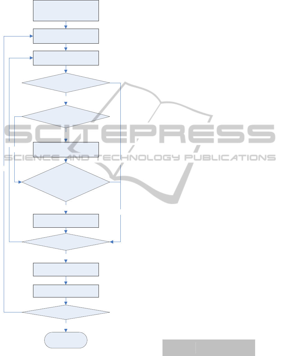
Compute initial dummy solution
and list of savings’ edges for
both edge directions
Sort the list of savings’ edges
with a biased random criterion
Assign bigger available vehicles
to each route
Unify routes
Is mergedCost = maxRouteLength?
Each route load can be assigned to a
candidate vehicle? (load = vCap)
Is empty the savings’ edge list?
Apply cache-based Local Search
Update best found solution
Is time < maxTime?
Each route has a candidate vehicle?
Y
N
Y
Y
Y
Extract a saving edge from the
list
N
N
N
Y
End
N
Figure 1: Overview of our approach.
appropriate dataset presented in (Marmion et al.,
2010) is related to our specific problem. The
experiments are based on a set of real instances
related to ACVRP (Fischetti et al., 1994). The
authors simulate the heterogeneous fleet over a
range of values for testing some operators on four
different algorithms. However, the proposed
benchmarks have only considered the effect of
variable cost on vehicles selection by ignoring the
different capacities. As a result, there is no specific
dataset for the above studied problem.
As the case of study, we used the information of
a food distribution company located in Barcelona,
Spain. The company has provided us with the
delivery address of their customers in six
independent days along with their demands for those
days. The transportation limits are defined inside of
the city borders (urban distribution).
The main interest of the company is to apply the
proposed approach to bigger datasets using a web
information tool. For this reason, the company just
compile the information during a short period (as a
sample) in order to produce a preliminary result. In
addition, the compiling process represented an
important investment of resources considering the
size of the company. Therefore on a daily basis, this
company receives requests from around 50
customers. This information serves as input to
manually design the company’s routing planning.
According to the size of the company it is not
possible to employ a person specialized in
mathematical software in order to apply exact
methods. Therefore they prefer to have an
approximated solution algorithm embed in a web
tool which could be used to give automatic solution
in little time.
There is a specific constraint: each vehicle must
visit all customers of a route in a maximum period
of 180 minutes. This route length restriction must to
include the travelling time and the service time. So
far, the company uses two types of vehicles, which
are described in the Table 1. The columns of this
table show the capacity (Q
k
) and quantity (m
k
) of
available vehicles for each type (k). Actually the
company used four vehicles, but they needed to
determine if it is possible to reduce the total routing
costs and also execute the same deliveries with
fewer routes.
Table 1: Composition of the current company fleet.
Vehicle Type
k
Q
k
m
k
1
20 2
2
30 2
We have used a map-location service, like
Google Maps to generate the asymmetric cost matrix
Multi-startApproachforSolvinganAsymmetricHeterogeneousVehicleRoutingProbleminaRealUrbanContext
23

between every pair of nodes (50 x 50 maximum
cells). Even when this kind of routing considers all
possible streets of the city, the cost matrix will only
represent the best travelling time between each two
nodes.
The main features of given six data instances are
summarized in the Table 2. On the first column, we
present the identification of each instance that
represents a day. The second column shows the
number of customers with demands. Third column is
the total demand. And the last column represents the
total service time of all the nodes on the instance.
As commented before, the company provides us
with the historic data of some of their service times
and routes. We have randomly generated the
respective values for the instances, using simulation
theory (Monte Carlo Simulation) and the provided
data. Then, we have defined that the service time for
each client follows a triangular distribution with min
= 1, max = 12 and mode = 3 minutes. This
distribution is often used to represent time in general
simulation models. However, the routes used differ
among all days. Notice that the company did not
save exact information of all their routes, even
within a whole day. Likely they do not apply any
specific routing method. A person in charge, who
tries to assign routes to all drivers, designs the
routing planning.
Table 2: General features of real instances.
Instance
(day)
Number of
Customers
Total
Requested
Demand
Total
Service
Time
(min)
A
40 53
163
B
50 75
213
C
40 60
163
D
39 54
159
E
40 57
162
F
18 28
75
5 NUMERICAL RESULTS
Our algorithm was implemented as a Java
application and used to run the six instances
described above on an Intel Xeon E5603 at 1.60 Ghz
and 8 GB of RAM. For each instance, a single run
with a total maximum time of 500 seconds was
employed. The limitation in computing time is due
to the fact that we wanted to obtain results in a
‘reasonable’ amount of time. We employ the
Random Number Generator (RNG) library for
Stochastic Simulation developed by researchers of
the Montreal University
(http://www.iro.umontreal.ca/~simardr/ssj/).
Table 3 shows the results obtained in
experiments. The first column shows the instance id;
the second, the number of routes defined in the
solution; the third column, the total travelling times
of routes; the fourth column, the total routing costs
considering the travelling times plus the service
times of the instance; and the last column, the
computational time needed to find the best solution.
The travelling costs on instances B and E
represent the higher values obtained. Both of them
travelling costs are bigger than the previously
commented restriction of 180 minutes. However,
this restriction is applied to the route duration and
also it considers the service time on each node. On
these two instances, the average total routing cost of
routes has to be considered. For this, the total
routing cost is divided by the number of routes on
the solution producing 134 and 174 minutes
respectively.
Notice that even when the running time is set to a
maximum limit of 500 seconds, the average time for
finding the best solutions is less than 131 seconds.
Table 3: Results of Best Solutions after 500 seconds
running.
Instance
(day)
Routes
Total
Travelling
Cost
(min)
Total
Routing
Cost
(min)
Time
(sec)
A
2
173 336 1.14
B
3
189 402 114.76
C
2
170 333 137.52
D
2
172 331 275.90
E
2
186 348 253.42
F
2
116 191 0.25
Average 2.17
167.67 323.50 130.50
In order to validate the solution quality of our
approach, we have compared our results against an
approximated value of the current total routing costs.
As we said before, the company does not have the
exact values of routing costs. However, they tend to
use all four vehicles as an attempt to reduce delivery
times, in an intuitive way. Therefore we have forced
our algorithm to use four vehicles in order to
produce a near value of current company solutions.
The output represents the best solution found in 500
seconds. We delivered the forced four-route solution
to the company in order to validate it with the real
planning, and we obtained a positive confirmation.
Table 4 presents the travelling times for each
ICORES2013-InternationalConferenceonOperationsResearchandEnterpriseSystems
24
scenario and the gap between these two solutions.
The difference between the approximated
company solutions and our approach results is
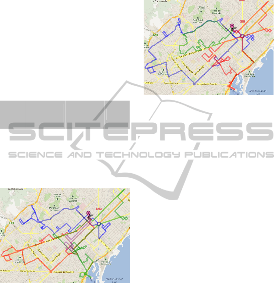
around 13%. In the next two images, we have
illustrated both routing solutions of the
approximated planning (Figure 2), and the new
proposed solution (Figure 3) for the instance B,
where the number of routes was reduced to 3. Notice
that the average number of routes of our approach is
around 2 which represents a considerable reduction
of the amount of routes.
Table 4: Comparison with extreme case using whole fleet
(four vehicles).
Instance
(day)
Best Costs
using 4 routes
(min)
(2)
Best Costs
(min)
(1)
GAP
(2-1)
A
192 173 -9.90%
B
205 189 -7.80%
C
206 170 -17.48%
D
190 172 -9.47%
E
211 186 -11.85%
F
153 116 -24.18%
Average
192.83 167.67 -13.45%
Figure 2: Approximated routing planning of the company
for instance B, using Google Maps.
6 CONCLUSIONS
In this paper, we have presented a multi-start
approach for solving the Asymmetric Heterogeneous
Vehicle Routing Problem (AHVRP) with service
time consideration and routes length restrictions.
The proposed approach integrates a randomized
heuristic approach with a local search. Our results
Figure 3: Designed routes in the proposed solution for
instance B, using Google Maps.
are based on data obtained from a distribution
company and we compare our solutions with an
approximation value of the actual ones implemented
by the company. These results revealed promising
improvements.
Through this experience it was possible to
support a food distribution company to: (a) realize
the current situation with quantitative methods; and
(b) improve their routing planning with a simple
approach. We used Monte Carlo Simulation to
complete the missing data from the company, and
obtain the information required for testing.
A popular way to evolve a study related to
savings algorithms is to propose new savings
definitions. The proposed definition of savings for
asymmetric VRPs could change in order to promote
other types of route constructions. Likely the
inclusion of other real constraints for urban
distribution is also being considered in the next steps
of our research, such as manage open routes and
balanced loads on routes. In fact this last restriction
is important because there are some routes with
fewer planned visits whereas others with more.
ACKNOWLEDGEMENTS
This work has been partially supported by the
Spanish Ministry of Science and Innovation
(TRA2010-21644-C03). It has been developed in the
context of the IN3-ICSO program and the CYTED-
HAROSA network (http://dpcs.uoc.edu).
Multi-startApproachforSolvinganAsymmetricHeterogeneousVehicleRoutingProbleminaRealUrbanContext
25

REFERENCES
Baldacci, R., Battarra, M., Vigo, D. 2008. Routing a
Heterogeneous Fleet of Vehicles. In The Vehicle
Routing Problem: Latest Advances and New
Challenges. B. Golden, S. Raghavan and E. E. Wasil,
Springer: 3-27.
Cáceres-Cruz, J., Lourenço, H., Juan, A., Grasas, A.,
Roca, M., Colome, R. 2012. Aplicación de un
Algoritmo Híbrido para la Resolución de un Problema
de Enrutamiento de Vehículos Heterogéneos en una
Empresa de Distribución. In Proceddings of Congreso
Español sobre Metaheurísticas, Algoritmos Evolutivos
y Bioinspirados (MAEB), 767-773. February 8-10.
Albacete, Spain.
Clarke, G., Wright, J. 1964. Scheduling of vehicles from
central depot to number of delivery points. Operations
Research, 12(4):568–581.
Dantzig, G. B., Ramser, J. H. 1959. The Truck
Dispatching Problem. Management Science 6:80–91.
Fischetti, M., Toth, P., Vigo, D. 1994. A branch-and-
bound algorithm for the capacitated vehicle-routing
problem on directed-graphs. Operations Research
42(5):846–859.
Juan, A. A., Faulín, J., Ruiz, R., Barrios, B., Caballe, S.
2010. The SR-GCWS Hybrid Algorithm for Solving
the Capacitated Vehicle Routing Problem. Applied
Soft Computing 10: 215–224.
Juan, A. A., Faulin, J., Jorba, J., Riera, D., Masip; D.,
Barrios, B. 2011. On the Use of Monte Carlo
Simulation, Cache and Splitting Techniques to
Improve the Clarke and Wright Savings Heuristics.
Journal of the Operational Research Society 62: 1085-
1097.
Laporte, G., Mercure, H., Nobert, Y. 1986. An exact
algorithm for the asymmetrical capacitated vehicle-
routing problem. Networks 16(1): 33–46.
Laporte, G. 2009. Fifty Years of Vehicle Routing.
Transportation Science 43(4): 408-416.
Li, F., Golden, B., Wasil, E. 2007. A record-to-record
travel algorithm for solving the heterogeneous fleet
vehicle routing problem. Computers & Operations
Research 34: 2734-42.
Marmion, M. E., Humeau, J., Jourdan, L., Dhaenens, C.
2010. Comparison of neighborhoods for the HFF-
AVRP, Computer Systems and Applications
(AICCSA), 2010 IEEE/ACS International Conference
on , pp.1-7, 16-19 May 2010.
Pessoa, A., Poggi de Aragão, M., Uchoa, E. 2008. Robust
Branch-Cut-and-Price Algorithms for Vehicle Routing
Problems. In The Vehicle Routing Problem: Latest
Advances and New Challenges. B. Golden, S.
Raghavan and E. E. Wasil, Springer: 297-325.
Rodríguez, A., Ruiz, R. 2012. A study on the effect of the
asymmetry on real capacitated vehicle routing
problems. Computers & Operations Research 39(9):
2142–2151.
Subramanian, A., Penna, P. H. V., Uchoa, E., Ochi, L. S.
2012. A hybrid algorithm for the heterogeneous fleet
vehicle routing problem. European Journal of
Operational Research 221: 285-295.
Toth, P., Vigo, D., 1999. A heuristic algorithm for the
symmetric and asymmetric vehicle routing problems
with backhauls. European Journal of Operational
Research 113: 528-543.
Vigo, D. 1996. A heuristic algorithm for the Asymmetric
Capacitated Vehicle Routing Problem. European
Journal of Operational Research 89: 108-126.
ICORES2013-InternationalConferenceonOperationsResearchandEnterpriseSystems
26
