Hybrid Particle Lattice Boltzmann Shallow Water

for Interactive Fluid Simulations

Jesus Ojeda

and Antonio Sus

ın

Dept. LSI, Universitat Polit

ecnica de Catalunya, Barcelona, Spain

Dept. MA1, Universitat Polit

ecnica de Catalunya, Barcelona, Spain

Keywords:

Fluid Simulation, Natural Phenomena, Physically based Animation.

Abstract:

We introduce a hybrid approach for the simulation of ﬂuids based in the Lattice Boltzmann Method for Shallow

Waters and particle systems. Our modiﬁed LBM Shallow Waters can handle arbitrary underlying terrain and

arbitrary ﬂuid depth. It also introduces a novel and simpliﬁed method of tracking dry-wet regions. Dynamic

rigid bodies are also included in our simulations using a two-way coupling. Certain features of the simulation

that the LBM can not handle, as breaking waves, are detected and automatically turned into splash particles.

Albeit we use a simple ballistic particle system, our hybrid method can handle more complex systems as SPH.

Both the LBM and particle systems are implemented in CUDA, yet dynamic rigid bodies are simulated in

CPU. We show the effectiveness of our method with various examples which achieve real-time on commodity

hardware.

1 INTRODUCTION

In the last years, professionals from real-time render-

ing and interactive ﬁelds have become more aware

of physically-based effects as new graphics hardware

can be used for such purposes. Among the most com-

mon features in actual computer games we ﬁnd parti-

cle systems, rigid bodies and ﬂuid simulations. Being

the last one the most complex and difﬁcult to achieve

in real-time. Moreover, the possibility of coupling all

these simulations opens a wide range for building rich

scenes with more interactivity.

Regarding ﬂuid simulations, the restrictions of the

equations and the extension of the simulations make

them difﬁcult to solve. Eulerian ﬂuid simulations

compute the ﬂuid properties at ﬁxed points in space,

distributed over a grid. On the other hand, Lagrangian

approximations evaluate the ﬂuid properties at points

that are advected with the ﬂuid itself. Whatever the

chosen method, the visualization of the ﬂuid is usu-

ally based on its surface. For great volumes of water,

their representation can be simpliﬁed to this bound-

ary, so the 3D simulation could potentially be reduced

to a 2D simulation of an evolving height ﬁeld.

Solving the 2D wave equation is a common tech-

nique to simulate ﬂuid surfaces as height ﬁelds, but

it can not resolve effects based on horizontal veloc-

ity ﬁelds as whirlpools. To account for this, a shal-

low water framework is preferred. Derived from the

more common Navier-Stokes equations, it is imple-

mented based on a discretization on time and space

over a grid. An alternative, less commonplace, deriva-

tion of these equations, but increasing in popularity,

is based on the Lattice Boltzmann Method, which

simpliﬁes the implementation, restricting the maxi-

mal wave speed.

A 2D heightﬁeld representation of a ﬂuid can not

account for many interesting phenomena that could

happen in a full 3D simulation, like breaking waves.

To improve this situation, we propose an implementa-

tion of an hybrid system that couples a Shallow Water

Lattice Boltzmann with particle systems in CUDA for

real-time ﬂuid surface simulation with the following

key features:

• Use of arbitrary underlying terrain.

• A method to maintain stability and to track dry-

wet regions in the simulation.

• Two-way simpliﬁed coupling with rigid body sim-

ulations using a proxy system.

• Breaking wave detection conditions.

• Full particle generation, simulation and reintegra-

tion with the heightﬁeld system.

Although we have used a ballistic particle system

for the present work, it is easily interchangeable with

217

Ojeda J. and Susín A..

Hybrid Particle Lattice Boltzmann Shallow Water for Interactive Fluid Simulations.

DOI: 10.5220/0004211302170226

In Proceedings of the International Conference on Computer Graphics Theory and Applications and International Conference on Information

Visualization Theory and Applications (GRAPP-2013), pages 217-226

ISBN: 978-989-8565-46-4

 2013 SCITEPRESS (Science and Technology Publications, Lda.)

other, more sophisticated methods, like SPH.

1.1 Related Work

A simple way to simulate water surfaces is based in

procedural methods, as those based in the Fast Fourier

Transform like (Tessendorf, 1999) or (Hinsinger

et al., 2002). These methods are well suited for the

generation of high resolution and large scale anima-

tions, and have been used extensively in commercial

products as movies or videogames; however, they are

not easily coupled with solid objects and are unable

to simulate eddies.

In computer graphics, (Kass and Miller, 1990)

were among the ﬁrst to use a shallow waters frame-

work implemented as a pipe model where adjacent

cells are connected by pipes, through which the ﬂuid

ﬂows. (O’Brien and Hodgins, 1995) extended that

pipe model, using particles for the splashes generated

from falling objects. More recently, (

St’ava et al.,

2008) ported this model to GPUs for the simulation

of hydraulic erosion. As an alternative, (Yuksel et al.,

2007) presented a novel approach using wave trains

on 2D particles to solve the wave equation. These

methods, however, can not simulate vortices or just

horizontal ﬂow.

On the other hand, the Shallow Water Equations

(SWE) can simulate these phenomena. In addition to

the heightﬁeld description of the ﬂuid surface, it also

simulates a 2D horizontal velocity ﬁeld. (Layton and

van de Panne, 2002) were the ﬁrst to introduce them

to the graphics ﬁeld. Among other works, (Th

urey

et al., 2007) used them to simulate breaking waves

and later were ported to CUDA by (Chentanez and

uller, 2010), coupling it with a particle system.

A Smooth Particle Hydrodynamics (SPH) system

can also be used to solve these equations. (Cords,

2007) coupled an SPHSW with the wave equation

to obtain higher detail ﬂuid surfaces. (Lee and Han,

2010) ported the SPHSW simulation to CUDA and

has already been extended by (Solenthaler et al.,

2011).

Yet another formulation can be stated with the Lat-

tice Boltzmann Method (LBM). The LBMSW deriva-

tion can be found in (Salmon, 1999) and has been

used in various scenarios. Among others, (Th

urey,

2007) coupled it with a full 3D LBM simulation and

(Th

ommes et al., 2007) used it to simulate the cur-

rents in the strait of Gibraltar. More recently, (Zhou,

2011) simpliﬁed the force terms of the formulation.

As the LBM is quite similar to a cellular automata,

it can be implemented in a parallel setting without

much effort with regard to other methods. There are

already GPU implementations as (Wei et al., 2004),

where it was adapted using textures; but more re-

cently, with the advent of general programmability of

GPUs we ﬁnd CUDA implementations like (T

olke,

2010) and (Obrecht et al., 2011). (Bailey et al., 2009)

proposed an alternative kernel implementation to re-

duce memory usage and (Geveler et al., 2010) tar-

geted multiple different parallel architectures using

higher-level libraries for solving the LBMSW model.

2 METHODOLOGY

The main steps our hybrid particle-LBM coupling ex-

ecutes for one time step (or render frame) can be sum-

marized, following the same order as the explanation

through this paper, as:

1. LBMSW ﬂuid simulation.

2. Rigid body simulation.

3. Two-way coupling of rigid bodies and LBMSW.

4. Particle generation and simulation.

5. Render

The ﬁrst step is to advance the LBMSW simula-

tion explained in Section 2.1. This takes into account

external forces and the dry-wet region tracking from

Section 2.2. Using any external package, as the Bullet

Physics library in our case, rigid bodies are simulated.

These are then coupled with the ﬂuid as presented in

Section 2.3. This two-way coupling affects the move-

ment of the dynamic objects but also modiﬁes the be-

haviour of the ﬂuid. Next, particles are generated and

simulated for all the ﬂuid regions the LBMSW can

not handle, as breaking waves. These particles sub-

tract some volume from the LBMSW in their genera-

tion and restore it back when they fall to the surface

again. Details about this process will be discussed in

Section 2.4. Finally, the render of the scene should

be done. Although we have implemented the render

phase with OpenGL, it is out of the scope of this pa-

per.

The mathematical formulation gives the basic un-

derstanding for the reproduction of our results but we

will provide more speciﬁc details about the CUDA

implementation in Section 3.

2.1 Lattice Boltzmann Shallow Waters

In contrast to other methods where a set of partial dif-

ferential equations is discretized and solved directly,

the Lattice Boltzmann Method already provides a dis-

crete model suitable for parallel computations using

only arithmetic operations. The ﬂuid is simulated by

particle distributions over a regular grid (distribution

GRAPP2013-InternationalConferenceonComputerGraphicsTheoryandApplications

218

functions d f s). The particle’s movement is restricted

to certain directions e

deﬁned by the Boltzmann dis-

cretization used.

Figure 1: D2Q9 model: nine velocity square lattice.

We use the D2Q9 model, pictured in Figure 1,

and assuming an adimensional parametrization as in

(Th

urey, 2007), the velocity vectors e

0..8

take the val-

ues: e

= (0,0)

, e

1,2

= (±1,0)

, e

3,4

= (0,±1)

and

5..8

= (±1, ±1)

The Lattice Boltzmann Equation, then, deﬁnes the

behaviour of the ﬂuid by the chosen collision oper-

ator. We employ here the common BGK operator

(Qian et al., 1992)

(x +e

∆t,t + ∆t) = f

(x,t) −ω( f

− f

) + F

, (1)

where f

is the d f for the e

direction, ω is the relax-

ation parameter, in close relation with the viscosity

of the ﬂuid, and f

is the local equilibrium distribu-

tion function, which deﬁnes the actual equations that

are being solved. The original SWE can be recovered

by applying Chapman-Enskog expansion if f

is de-

ﬁned like in, e.g., (Salmon, 1999)

(h,u) =

(



1 −

gh −



, i = 0,



·u

·u)

−



, i 6= 0,

(2)

where λ

= 1 for i = 1..4 and λ

= 1/4 for i = 5..8. g

is the gravity and h and u are the macroscopic ﬂuid

properties; height level from the underlying terrain

and velocity, respectively, calculated as

h(x,t) =

∑

, (3)

u(x,t) =

∑

. (4)

From Equation 1, F

are the external forces applied

to the LBMSW. In contrast to how these forces are

applied in, e.g., (Th

ommes et al., 2007) or (Geveler

et al., 2010); (Zhou, 2011) stated them with simpler

arithmetic operations as

= X

+ Z

. (5)

From a constant underlying terrain z

(x) deﬁned as a

heigthﬁeld, X

is the force caused by its slope as

(

(x + e

∆t) −z

(x)], i = 1..4,

0, otherwise,

(6)

with

h = [h(x + e

∆t,t) + h(x,t)]. (7)

internalises other forces F, as friction, wind or the

Coriolis effect, deﬁned as

(

0, i = 0,

, i 6= 0,

(8)

where α is a Cartesian index and Einstein summation

convention is used. The same can be applied to e

We only consider the friction with the underlying ter-

rain, so F

is deﬁned as

= C

√

, (9)

where β is the other Cartesian index and C

is the ter-

rain friction coefﬁcient, deﬁned as a constant. u

and

are the components of the ﬂuid velocity in the α

and β directions, respectively.

As boundary conditions, we use a no-slip bound-

ary which provides normal and tangential velocities

equal to 0. For the LBM, this type of boundary is eas-

ily implemented as a bounce-back rule: the d f s that

should be streamed from boundary cells are just in-

verted as

(x,t +∆t) = f

(x,t), (10)

where f

is the d f in the opposite direction of f

, i.e.,

= −e

Additionally, we use for the rest of the paper the

value η deﬁned as

η(x,t) = h(x,t) + z

(x). (11)

2.2 Dry-wet Region Tracking

In order to be able to track dry regions, i.e., cells

that do not contain ﬂuid, we modify the original algo-

rithm. We deﬁne a threshold ε as the minimal height

a cell must satisfy to be considered a Fluid cell. Af-

ter an iteration of the LBM has been executed, we

must look for cells whose level has dropped below

the threshold. For all the found cells, we must tag

them as Empty. In order to not lose ﬂuid mass, we

also distribute the remainder of the ﬂuid between the

Fluid neighbours favoring the direction of the under-

lying terrain gradient as follows:

(x + e

∆t) = f

(x + e

∆t) + h(x) ·(ζ

/ζ

total

), (12)

where ζ

total

is the sum of all weights ζ

, which are

computed as











−(∇z

·e

) if −(∇z

·e

) > 0 and cell at

(x + e

) is a Fluid one,

0 otherwise.

(13)

HybridParticleLatticeBoltzmannShallowWaterforInteractiveFluidSimulations

219

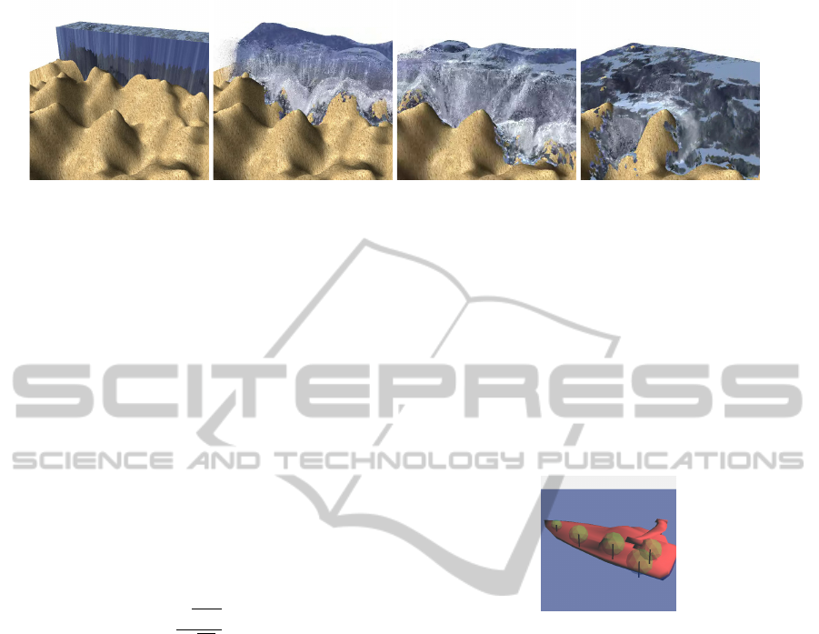
Figure 2: Image stills from the breaking dam over noisy ground example. Using values of ε = 0.1 and ϕ = 0.95.

Seamlessly, we search also for Fluid cells whose

ﬂuid level is above the threshold and whose neigh-

bours are Empty cells. We tag these Empty cells as

Fluid, in order to allow the advance of the ﬂuid from

the Fluid tagged cell.

This simple addition enables for the tracking of

dry-wet regions, but yet one more limitation of the

LBM has to be circumvented to allow fully functional

simulations. This comes from Equation 4, where, as

the ﬂuid level goes down, the velocities can grow very

large and lead to inevitable instabilities. In contrast

to (Geveler et al., 2010), where they worked around

this by using a modiﬁed minmod ﬂux limiter, we

have used a more direct approach. It is known that

the LBMSW is suitable for subcritical ﬂows (Zhou,

2004), and this condition is given by the Froude num-

ber which relates the characteristic velocity of the

ﬂuid to a gravitational wave velocity

Fr =

√

u ·u

√

, (14)

which is deﬁned as Fr < 1 for subcritical ﬂows.

We deﬁne an upper limit parameter ϕ for that ratio.

When, due to low ﬂuid height, the ratio does not hold,

we compute a new suitable velocity u for the ﬂuid

and replace the d f s of the cell with new ones com-

puted from Equation 2. Also, we can further use this

condition to dampen high velocities through the full

body of ﬂuid and ensure a stable simulation.

Although not physically correct, this method en-

sures stability in a similar fashion to the Smagorinsky

method (Hou et al., 1996), it changes the local viscos-

ity of the ﬂuid and dampens high velocities, as can be

seen in Figure 2. The Smagorinsky method can addi-

tionally be applied here for improved stability condi-

tions.

2.3 Two-way Coupling of Dynamic

Objects

In this section we explain how dynamic objects,

more speciﬁcally rigid bodies, are introduced to the

LBMSW simulation. We propose the use of a proxy

model to decouple the complexity of the interaction

of the ﬂuid with the object mesh, in contrast to (Chen-

tanez and M

uller, 2010), where they use a tessellated

mesh to the level of using triangles of areas similar to

∆x

, from the ﬂuid simulation.

Our proxy model is composed of a set spheres

with some properties deﬁned, and can be under-

stood as a rough discretization of the object mesh.

The properties deﬁned for the spheres are the ra-

dius r, the position p = (p

, p

)

and a normal

n = (n

)

. During the simulation, the spheres

will also hold a velocity v = (v

)

Figure 3: Sphere discretization example for a boat model.

The spheres are positioned and sized within the model, their

normal vectors represented by the black short lines.

For our examples, we have used manually dis-

cretized models, as the boat in Figure 3. Depend-

ing on the number of spheres, their size and position

within the model, the simulation becomes more ac-

curate but also more expensive. For a regular spaced

discretization with spheres of radius r < ∆x/2 we ob-

tain similar visual results to (Chentanez and M

uller,

2010).

2.3.1 Fluid to Solid

For the implementation of the ﬂuid to solid coupling

we follow the path of (Yuksel et al., 2007) and (Chen-

tanez and M

uller, 2010). There are three major forces

a ﬂuid can induce to a solid body: buoyancy, drag and

lift. They will be computed at the position of each

sphere of the proxy object. The values needed from

the ﬂuid will be bilinearly interpolated. We assume

that the simulation plane is xz, thus ˆy = (0, 1,0)

The buoyancy force points upward and is propor-

tional to the weight of the displaced ﬂuid, we can de-

GRAPP2013-InternationalConferenceonComputerGraphicsTheoryandApplications

220

ﬁne it for sphere i as

buoy

(

0 if S

−S

> η

gρV

sub

ˆy otherwise,

(15)

where, η

is the water level at the sphere position,

is the sphere radius, S

is the y coordinate of the

location of the sphere, ρ is the density of the ﬂuid and

sub

is the volume of the submerged part of the sphere

calculated as

sub

top

−S

π(S

−x

)dx, (16)

with top = (η

−(S

−S

)).

Drag force is a resistive force and is dependent on

the actual velocity of the obstacle with regard to the

ﬂuid. Lift is a force perpendicular to the oncoming

ﬂow direction, it contrasts with the drag force as that

one is parallel to the ﬂow direction. For sphere i, they

are deﬁned as

drag

= −

rel

, (17)

li f t

= −

rel



rel

×u

rel

×u

rel



(18)

where C

and C

are the drag and lift coefﬁcients,

rel

is the relative velocity of the sphere with respect

to the ﬂuid, S

is the normal deﬁned for the sphere

and A

is the area of the circle that cuts the sphere at

water level η

The forces are ﬁnally added to the ith sphere. The

rigid body simulator will take care of the evolution of

the proxy model and will provide the corresponding

transform which will be applied in the render phase.

2.3.2 Solid to Fluid

In this case, the rigid body will modify the behaviour

of the ﬂuid. As before, the computations are done

per sphere. To change the ﬂuid correctly, we get the

velocity of the obstacle for the ith sphere as v and

the difference between the submerged height of the

sphere and the ﬂuid level as depth. We compute the

following values

decay = exp(−depth), (19)

= decay ·C

dis

·depth, (20)

= decay ·C

ad p

·v, (21)

and input these h

and u

into the LBM equilibrium

distribution, Equation 2, updating the previous d f s as

= f

−h

= f

+ f

) +

)

where w







5 i = 1..4,

20 i = 5..8.

(22)

The values of w

are calculated from the contribu-

tion each e

gives on the D2Q9 model (He and Luo,

1997). With this computation we push the ﬂuid the

obstacle is displacing to the neighbour cells, taking

into account in this process the obstacle velocity. Ad-

ditionally, to avoid high differences between contigu-

ous points of the ﬂuid mesh, we distribute the h

and

among the nearest cells using linear interpolation.

Figure 4: A buoy is being dragged by the ﬂuid (left). The

boat introduces some new ﬂuid waves at its tail as a result

of the coupling (right).

decay takes into account the depth the sphere is at

and limits accordingly the effect it has over the ﬂuid

surface. C

dis

and C

ad p

are parameters in the range

[0,1] that allow to dampen the effect of the coupling

as desired. We have used the values C

dis

= 0.8 and

ad p

= 0.5 for the examples of Figure 4.

2.4 Particle Systems Coupling

The LBMSW model described so far is only capa-

ble of representing ﬂuids as heightﬁelds. It is lim-

ited in the kind of phenomena that can be simulated,

e.g., breaking waves can not be resolved. In order to

deal with this restriction, we have coupled it with a

ballistic particle system and adapted the detection of

breaking waves and generation of the respective par-

ticles from (Chentanez and M

uller, 2010). Because

there is no silver bullet for every situation when par-

ticles should be generated, they proposed also meth-

ods to detect when to generate (and how to initialize)

particles for the interaction with obstacles and terrain

discontinuities like waterfalls, which could also be

adapted to our system. As these methods are tailor-

made for each situation, we restrict ourselves to the

breaking wave example. In contrast, we will present

an implementation that allows alternative particle sys-

tems like SPH with minor changes in Section 3.

To be consistent with the LBM, we use the same

adimensional parametrization, so ∆x and ∆t are con-

sidered to be equal to 1 inside the iteration. For ren-

der purposes, a redimensionalization must be applied,

however.

HybridParticleLatticeBoltzmannShallowWaterforInteractiveFluidSimulations

221

2.4.1 Breaking Wave Detection

Waves that would break in a full 3D simulation just

produce singular waves due to numerical instability

in a Shallow Waters simulation. The detection of

this situation for a given cell (i, j) is done via three

parametrized conditions:

k∇η

i, j

k > Φg, (23)

i, j

−η

i, j

> Ψ, (24)

∇

i, j

< ϒ, (25)

where η

i, j

is the ﬂuid height in the previous time

step and Φ, Ψ and ϒ are parameters, which should

be tailored per scene, and more speciﬁcally by its

scale. Equation 23 ensures the wave is steep enough

to break. Equation 24 requires that the cell is part

of the front of the wave and it is raising fast, intro-

ducing a comparison with the previous value of ﬂuid

height. Finally, Equation 25 makes sure particles are

only generated near the top of the wave.

The computation of ∇η

i, j

is done using the maxi-

mum among the one-sided derivatives

∇η

i, j

max(|η

i+1, j

−η

i, j

|,|η

i, j

−η

i−1, j

∆x

max(|η

i, j+1

−η

i, j

|,|η

i, j

−η

i, j−1

∆x

. (26)

Similarly, ∇

i, j

is computed using central differ-

ences as

∇

i, j

i+1, j

+ η

i−1, j

+ η

i, j+1

+ η

i, j−1

−4η

i, j

∆x

(27)

If all three conditions are met, the next step will

generate and initialize particles for the given cell. The

total volume V

total

the added particles will subtract

from the LBMSW is proportional to k∇η

i, j

k−Φg and

can be controlled introducing a new parameter θ, as

total

= θ(k∇η

i, j

k−Φg). (28)

2.4.2 Particle Generation

For each cell detected in the previous step, a num-

ber of particles will be generated for the volume of

Equation 28. For a particle of radius r, its volume is

πr

The particles are positioned within a cell-centered

rectangle of width equal to the LBMSW cell width

and height V

total

as shown in Figure 5. This rectangle

is oriented with the opposite direction of the gradient

computed in Equation 26.

The particle velocities in the xz plane are deﬁned

by the wave speed as in (Th

urey et al., 2007) and the

y component can be deﬁned as a fraction of the height

(

i, j)

∆x

−

∇η

(i, j)

k∇η

(i, j)

Figure 5: For breaking wave detected particles, they are

placed within the red rectangle in their generation step.

differences from Equation 24 as

−∇η

i, j

√

k∇η

i, j

, (29)

= λ

(η

i, j

−η

i, j

), (30)

where λ

controls the fraction. We have used here a

value of λ

= 0.1.

Additionally, we lightly perturb the velocity of

each particle and jitter their initial positions between

[

−∆x

∆x

] in the gradient direction. These little pertur-

bations add variation and result in less uniform, more

chaotic, particle movement.

The total volume the particles supply must be sub-

tracted from the LBMSW, as well as the momentum

they get. We do this by computing the equilibrium

distribution function from Equation 2; using as input

values V

total

and the xz velocity components from the

particle velocities, prior to the perturbations we ap-

ply. These newly computed equilibrium d f s will be

subtracted from the cell’s original d f set as

= f

− f



total

∆x



. (31)

As said previously, particles are not restricted to

be generated only from the detected breaking waves

of the previous step. We can generate and initial-

ize particles with other requirements in mind, like a

faucet pouring ﬂuid into a basin as demonstrated by

Figure 6.

Figure 6: Particles generated in middle air (like a heavy rain

or some pipe open tab), integrated afterwards to the bulk of

the ﬂuid. After a few seconds, the level of the LBMSW is

effectively raised.

2.4.3 Particle Reintegration

Finally, the particles must be reintegrated to the

LBMSW when they hit the surface of the ﬂuid, i.e.,

GRAPP2013-InternationalConferenceonComputerGraphicsTheoryandApplications

222

≤ η

i, j

. The volume the particles carry, as well as

their momentum, must be absorbed by the cell they

fall on.

As the LBMSW has no explicit method to input

vertical velocities, we introduce an interpolation for

the absorption of the volume of the particle among the

cell’s d f s. This interpolation is based on the terminal

speed the particle could achieve, deﬁned as

8rg

, (32)

where C

is the drag coefﬁcient. We normalize the

particle’s vertical speed with v

and clamp the result

to the range [0,1], as χ = clamp(v

,0, 1).

Taking into account the previous consideration,

we calculate f

eqχ

= f



∆x



, (33)

and we can ﬁnally update the d f s of the cell using the

following computations

= f

+ (1 −χ) · f

eqχ

, (34)

= f

+ f



∆x

+ χ f

eqχ



. (35)

Similarly to the obstacle to ﬂuid coupling from

Section 2.3.2, using the interpolation with the ter-

minal speed, the added volume is pushed from the

cell’s center to its neighbours with more energy, the

faster the particle drops. Figure 2 shows how particles

generated from a breaking dam wave are reintegrated

even in dry sections and Figure 6 shows how the water

level of a basin is effectively raised from the mid-air

dropped particles.

3 IMPLEMENTATION DETAILS

In this section we give some implementation details of

the Particle-LBMSW coupling. As there is no simple

way to maintain a dynamic data structure for the par-

ticles, i.e., particles should be created and destroyed

on the ﬂy; we have resorted to a ﬁxed number of parti-

cles from the beginning of the simulation. In addition

to the usual particle properties as position and veloc-

ity, we add two more: a TTL (time-to-live) value and

an active (ACTIVE/INACTIVE) ﬂag. We will explain

their use in the particle-related functions.

In Algorithm 1 we show high-level pseudo-code

for the full simulation. All CUDA functions are ker-

nels, except the sort, remove and preﬁx sum parallel

operations, which are provided by the Thrust library.

There are kernels that are only targeted to a limited

Algorithm 1: Full per frame hybrid Particle-LBMSW high-

level algorithm.

dt = (∆t) frame time step (16ms)

dt’ = (∆t

) LBM dimensional time step

foreach(frame) {

//CPU

ObstacleSimulation();

ObstacleFluidCoupling();

//CUDA

ReintegrateParts_S1();

sort_tuples();

remove_nonValidTuples();

prefix_sum_tuples();

ReintegrateParts_S2();

for(i=0; i<dt; i+=dt’) {

LBM_stream_collision();

LBM_applyForce();

upd_CellTags_pre();

upd_CellTags_Fluid();

upd_CellTags_Empty();

}

computeLBM_GradLaplacian();

sort_particlesByTTL();

stepParticles();

detectBreakingWaveCells();

prefix_sum_NeededPartsPerCell();

initParticles();

//Render

}

group of cells or particles; they provide an early exit

condition for the elements that are not to be changed.

Below, we will explain the different kernels, starting

from the LBM simulation to the Particle coupling at

last.

The LBM core simulation, executed in the

LBM stream collision kernel is basically the same as

previous LBM implementations in CUDA like, e.g.,

(Geveler et al., 2010), (T

olke, 2010) or (Obrecht et al.,

2011); using the BGK collision operator instead of

the MRT one. This is done in an inner loop, as the

∆t

for the LBM is quite smaller than the ∆t of the

frame and depends on the parametrization used. In

contrast to (Bailey et al., 2009), where they proposed

an A-A memory access pattern to reduce memory re-

quirements, we have used an A-B memory access pat-

tern; there are two arrays for the d f s in memory and

they are interchanged after each iteration inside the

for loop. The reason for this choice is the additional

operations we are doing, they would have required to

double the kernels, as the A-A memory access pat-

tern needs two kernels just for the core simulation.

Nevertheless, we use separated arrays for each d f , in

order to ensure coalesced memory accesses like pre-

vious works.

HybridParticleLatticeBoltzmannShallowWaterforInteractiveFluidSimulations

223

The LBM applyForce kernel adds the force terms

from Equation 5 for the underlying slope and friction.

The three kernels upd CellTags * are the ones

responsible for the actual Dry-Wet region tracking.

Fluid cells that have a height above the threshold

ε must convert their Empty neighborhood to Fluid

in order to allow the ﬂuid to advance. Seamlessly,

Fluid cells with a height below the threshold must

be changed back to Empty. As CUDA executes by

warps inside blocks, we could fall into race condi-

tions in this change of type for the cells. To solve

this problem, we have to serialize the reﬂaging opera-

tions, thus the three kernels. upd CellTags pre checks

the height of the cells against the threshold and pre-

ﬂags them with an additional type if necessary: to-

beFluid or tobeEmpty. Next, we change the type of

the cells conservatively, ﬁrst the Fluid-to-be ones and

then the Empty ones. This way, we ensure no cells are

changed prematurely if they should be needed in the

next iteration.

Then, the computation of the gradient and lapla-

cian of the ﬂuid height is done for further use in the

breaking wave detection kernel.

The particles are then sorted by their TTL in as-

cending order. The particle simulation is advanced in

stepParticles, depending on the chosen particle sys-

tem. For a ballistic particle system, the velocity and

position of the particles are updated ignoring possi-

ble interaction between particles. The particles’ TTL

are also updated, subtracting the current ∆t. Their sta-

tus is also updated to ACTIVE. If a particle has died

(TTL ≤ 0) before being reintegrated, we let them be

ACTIVE but out of view. We can use this same be-

haviour for particles exiting the domain. This ensures

we don’t lose mass because of dead particles in the

particle generation step.

From the previously computed gradient and lapla-

cian and Equations 23 to 24 we detect the cells that

have a breaking wave. Each cell will output the

needed particle count that it needs. Then, with a

preﬁx sum operation we can obtain an accumulated

sum of the needed particles. We can use the result

of this accumulated sum as the index at the particle

array for which each cell will take their needed parti-

cle count. As particles have been sorted by TTL, we

ensure the particles ﬁrst taken in this step are those

who had a lower TTL. Unfortunately, if more particles

are needed than those with a TTL = 0, the next with

lower TTL will be taken. With a bad parametriza-

tion this can lead to artifacts, as disappearing parti-

cles from frame to frame as they are needed. init-

Particles will, then, initialize the particles needed for

each cell as explained in Section 2.4.2, marking them

as ACTIVE2 which ensures they are alive at least for

a frame. Their TTL is also set up as the maximum

allowed time to live for a particle, which is a user-

deﬁned parameter. For particles that were previously

marked as ACTIVE, no ﬂuid will be subtracted from

the LBMSW, ensuring no mass loss; thus, only IN-

ACTIVE particles will take ﬂuid from the LBMSW.

Needless to say, these steps for the detection and ini-

tialization of particles can be changed or improved to

take into account more situations as those described

in (Chentanez and M

uller, 2010).

Finally, although we have written it as one of the

ﬁrst steps in Algorithm 1, the particles are reintro-

duced. Only ACTIVE particles will be looked for.

For these particles, the reintegration should be as

easy as the explanation from Section 2.4.3 but, as we

can’t be sure how many particles can fall in a cell

at once, we should use atomic operations in the up-

date of the cell’s d f s. As our hardware, a GTX280,

does not support these operations for ﬂoat variables,

we had to solve it from another perspective: Rein-

tegrateParts S1 relates which particles have fallen in

which cells and how many there are for each cell;

from the cell point of view, ReintegrateParts S2 will

gather the fallen particles and update the local d f s. In

order to do so, for each particle, S1 will write a tuple

associating the cell id (the cell’s position in a linear

memory array) with the particle id, as well as the par-

ticle count for each cell (using integer atomics). Par-

ticles not to be reintegrated are associated to a fake

cell, in this case we use the cell 0 that we ensure is a

Boundary cell for all examples. Sorting the tuples by

the cell id, removing those with the fake cell id and

doing a preﬁx sum on the particle-in-cell count will

lead us to the cells having the index where their par-

ticle count starts in the tuple array. S2 will, for each

cell, take their counted fallen particles and reintegrate

them, marking them as INACTIVE with TTL = 0.

While the rigid body simulation is done in CPU,

we can only update the values as in Section 2.3 using

the CUDA memory arrays (not the opaque CUDA Ar-

ray handlers) mapped to CPU memory space.

As all the data needed is already in the GPU,

we use Vertex Array Buffers to interoperate with

OpenGL in the render phase.

4 RESULTS AND DISCUSSION

We have tested our implementation both on CPU with

OpenMP and GPU with CUDA, timings shown in Ta-

ble 1 for various examples. Our test system was an In-

tel Core2Duo E8400 with 4GB of RAM memory and

a Nvidia GTX280 running Ubuntu 11.10. We have

used the Bullet Physics library for the simulation of

GRAPP2013-InternationalConferenceonComputerGraphicsTheoryandApplications

224

Table 1: Timing per frame for various examples in milliseconds; the number in the name of the example indicates the total

number of particles used, where k = 2

. LBMSW includes the LBM simulation, as well as the dry-wet region tracking.

Solids accounts for the 2-way coupling of dynamic rigid bodies. PGen, PSim and PReint are the timings for the generation and

initialization, simulation and reintegration of the particles respectively. We have extracted the timings for the sort operation

from the Thrust library in Psort and PReint sort, as they do not depend directly on the other steps but have a signiﬁcant impact

on the results, more heavily on the CPU version. Psort is for the sorting of particles by their TTL. PReint sort is the sort of

the (cell id, particle id) tuples.

Total LBMSW Solids Psort PGen PSim PReint PReint sort

CPU

boat 10.78 10.69 0.09 0.00 0.00 0.00 0.00 0.00

buoy 10.91 10.85 0.06 0.00 0.00 0.00 0.00 0.00

drop 32k 372.96 9.97 0.00 214.56 1.16 1.46 31.50 114.31

drop 128k 1635.36 9.75 0.00 1001.35 2.09 2.79 114.92 504.46

wave 32k 410.88 9.62 0.00 224.04 3.68 4.85 32.58 136.11

wave 128k 1694.87 9.62 0.00 1007.30 3.37 10.71 117.51 546.36

GPU

boat 0.82 0.35 0.47 0.00 0.00 0.00 0.00 0.00

buoy 0.87 0.35 0.52 0.00 0.00 0.00 0.00 0.00

drop 32k 14.30 0.35 0.00 7.03 0.45 0.10 1.24 5.13

drop 128k 23.50 0.34 0.00 10.71 0.41 0.14 1.75 10.15

wave 32k 15.28 0.36 0.00 7.26 0.99 0.12 1.32 5.23

wave 128k 25.71 0.36 0.00 11.21 1.42 0.32 2.01 10.39

wave 256k 34.39 0.37 0.00 16.45 1.18 0.54 2.55 13.30

wave 512k 54.84 0.36 0.00 27.76 1.04 0.81 2.97 21.90

wavegr 64k 18.79 0.39 0.00 9.48 1.18 0.18 1.64 5.92

the rigid bodies and the Thrust library for parallel op-

erations like sort or preﬁx sum. The CUDA version

used was 4.1. The size of the grid used throughout

the examples is set to 128x128 and we ﬁx the time

step for each frame to ∆t = 16ms. For the boat and

buoy scenes, the particle coupling was deactivated to

allow us a better timing. For the same reason, for the

wave examples, the object coupling was deactivated.

The wavegr example is basically the same as the oth-

ers, a breaking wave generated from a breaking dam,

but in this case the rest of the domain is totally empty

as shown in Figure 2.

Although a direct comparison with (Chentanez

and M

uller, 2010) would not be totally fair because

of the difference in the hardware and their lack of im-

plementation details, at least for the particle simula-

tion in CUDA, we think that our LBM-based hybrid

system is a great alternative up to the challenge for

real-time ﬂuid simulations.

The hardware used has severely limited us. To en-

sure all the particles were reintroduced correctly with-

out loss mass and because the GTX280 had no sup-

port for ﬂoat atomic operations, we had to separate

the reintroduction step in two kernels plus some other

Thrust powered operations; the particles are not di-

rectly reintroduced but gathered by the cells. These

additional operations add more time to the processing

of the particles than what it should be needed with

more modern hardware.

Nevertheless, we have shown that a coupling of

LBMSW with a particle system is feasible for higher-

detail ﬂuid simulations. The particle system, how-

ever, is not limited to the ballistic version used in

here. While the coupling should be the same, i.e.,

generation and reintegration, TTL of particles and ac-

tive ﬂag; the simulation and behaviour of the particles

can be deﬁned alternatively. A CUDA implementa-

tion of SPH as in (Goswami et al., 2010) could be

easily adapted to our hybrid system and is part of fu-

ture work.

One limitation our system has, however, is the

sudden disappearance of particles due to high de-

manding simulations, i.e., more particles are needed

per frame than what is available. It will be interesting

to look at Level-Of-Detail techniques that allow to re-

lax this situation, if more particles than available are

needed, the ones actually being active could be rep-

resented with simpler primitives, grouping near par-

ticles, etc. Alternatively, it also would be worth in-

vesting in some technique that tries to prioritize the

preservation of visible particles, i.e., those that fall in

the actual view frustum.

Although we have not explained how the visual-

ization is done, the render of the ﬂuid is based in tri-

angle meshes in OpenGL. This can provoke some mi-

nor visual artifacts in the dry-wet region boundaries,

which should also be considered.

Other future work also includes the use of a rigid

body simulation totally in the GPU, as well as im-

prove the detection conditions for breaking waves.

Other particle generation conditions should be further

researched to broaden the use of this method.

HybridParticleLatticeBoltzmannShallowWaterforInteractiveFluidSimulations

225

ACKNOWLEDGEMENTS

With the support of the Research Project TIN2010-

20590-C02-01 of the Spanish Government.

REFERENCES

Bailey, P., Myre, J., Walsh, S., Lilja, D., and Saar, M.

(2009). Accelerating lattice boltzmann ﬂuid ﬂow sim-

ulations using graphics processors. In International

Conference on Parallel Processing, pages 550 –557.

Chentanez, N. and M

uller, M. (2010). Real-time simulation

of large bodies of water with small scale details. In

Proc. ACM SIGGRAPH/Eurographics Symposium on

Computer Animation (SCA), pages 197–206.

Cords, H. (2007). Mode-splitting for highly detailed, in-

teractive liquid simulation. In Proceedings of the

5th international conference on Computer graphics

and interactive techniques in Australia and Southeast

Asia, GRAPHITE ’07, pages 265–272, New York,

NY, USA. ACM.

Geveler, M., Ribbrock, D., G

oddeke, D., and Turek, S.

(2010). Lattice-boltzmann simulation of the shallow-

water equations with ﬂuid-structure interaction on

multi- and manycore processors. In Keller, R.,

Kramer, D., and Weiss, J.-P., editors, Facing the

multicore-challenge, pages 92–104. Springer-Verlag.

Goswami, P., Schlegel, P., Solenthaler, B., and Pajarola,

R. (2010). Interactive SPH simulation and ren-

dering on the GPU. In Proceedings ACM SIG-

GRAPH/Eurographics Symposium on Computer An-

imation, pages 55–64.

He, X. and Luo, L. S. (1997). Theory of the lattice Boltz-

mann method: From the Boltzmann equation to the

lattice Boltzmann equation. Phys. Rev. E, 56:6811–

6817.

Hinsinger, D., Neyret, F., and Cani, M.-P. (2002). Interac-

tive animation of ocean waves. In Proceedings of the

2002 ACM SIGGRAPH/Eurographics symposium on

Computer animation, SCA ’02, pages 161–166, New

York, NY, USA. ACM.

Hou, S., Sterling, J., Chen, S., and Doolen, G. D. (1996). A

Lattice Boltzmann Subgrid Model for High Reynolds

Number Flows. Fields Institute Communications,

6:151–166.

Kass, M. and Miller, G. (1990). Rapid, stable ﬂuid dynam-

ics for computer graphics. In Proceedings of the 17th

annual conference on Computer graphics and interac-

tive techniques, SIGGRAPH ’90, pages 49–57, New

York, NY, USA. ACM.

Layton, A. T. and van de Panne, M. (2002). A nu-

merically efﬁcient and stable algorithm for animat-

ing water waves. The Visual Computer, 18:41–53.

10.1007/s003710100131.

Lee, H. and Han, S. (2010). Solving the shallow water

equations using 2d sph particles for interactive appli-

cations. The Visual Computer, 26:865–872.

Obrecht, C., Kuznik, F., Tourancheau, B., and Roux, J.-

J. (2011). A new approach to the lattice boltzmann

method for graphics processing units. Computers &

Mathematics with Applications, 61(12):3628 – 3638.

O’Brien, J. F. and Hodgins, J. K. (1995). Dynamic simula-

tion of splashing ﬂuids. In Proceedings of the Com-

puter Animation, CA ’95, pages 198–. IEEE Com-

puter Society.

Qian, Y. H., D’Humi

eres, D., and Lallemand, P. (1992).

Lattice BGK models for Navier-Stokes equation. EPL

(Europhysics Letters), 17(6):479.

Salmon, R. (1999). The lattice boltzmann method as a ba-

sis for ocean circulation modeling. Journal of Marine

Research, 57(3):503–535.

Solenthaler, B., Bucher, P., Chentanez, N., M

uller, M., and

Gross, M. (2011). SPH Based Shallow Water Simula-

tion. In Bender, J., Erleben, K., and Galin, E., editors,

VRIPHYS 11: 8th Workshop on Virtual Reality Inter-

actions and Physical Simulations, pages 39–46, Lyon,

France. Eurographics Association.

Tessendorf, J. (1999). Simulating ocean water. SIGGRAPH

course notes.

ommes, G., Sea

ıd, M., and Banda, M. K. (2007). Lat-

tice boltzmann methods for shallow water ﬂow appli-

cations. International Journal for Numerical Methods

in Fluids, 55(7):673–692.

urey, N. (2007). Physically based Animation of Free Sur-

face Flows with the Lattice Boltzmann Method. PhD

thesis, Dept. of Computer Science 10, University of

Erlangen-Nuremberg.

urey, N., M

uller-Fischer, M., Schirm, S., and Gross, M.

(2007). Real-time breaking waves for shallow water

simulations. In Computer Graphics and Applications,

2007. PG ’07. 15th Paciﬁc Conference on, pages 39

–46.

olke, J. (2010). Implementation of a lattice boltzmann ker-

nel using the compute uniﬁed device architecture de-

veloped by nvidia. Computing and Visualization in

Science, 13:29–39. 10.1007/s00791-008-0120-2.

St’ava, O., Bene

s, B., Brisbin, M., and K

riv

anek, J.

(2008). Interactive terrain modeling using hydraulic

erosion. In Proceedings of the 2008 ACM SIG-

GRAPH/Eurographics Symposium on Computer An-

imation, SCA ’08, pages 201–210, Aire-la-Ville,

Switzerland, Switzerland. Eurographics Association.

Wei, X., Li, W., Mueller, K., and Kaufman, A. (2004). The

lattice-boltzmann method for simulating gaseous phe-

nomena. Visualization and Computer Graphics, IEEE

Transactions on, 10(2):164 –176.

Yuksel, C., House, D. H., and Keyser, J. (2007). Wave par-

ticles. ACM Trans. Graph., 26(3).

Zhou, J. G. (2004). Lattice Boltzmann Methods for Shallow

Water Flows. Springer.

Zhou, J. G. (2011). Enhancement of the labswe for shal-

low water ﬂows. Journal of Computational Physics,

230(2):394 – 401.

GRAPP2013-InternationalConferenceonComputerGraphicsTheoryandApplications

226