
Hybrid Iterated Kalman Particle Filter for Object Tracking Problems
Amr M. Nagy
1
, Ali Ahmed
2
and Hala H. Zayed
1
1
Faculty of Computers and Informatics, Benha University, Banha ElGadeda, Benha, Egypt
2
Faculty of Computers and Information, Menofia University, Shubin el Kom, Menufia, Egypt
Keywords:
Kalman Filter, Particle Filter, Nonlinear/Non-Gaussian, Object Tracking.
Abstract:
Particle Filters (PFs), are widely used where the system is non Linear and non Gaussian. Choosing the im-
portance proposal distribution is a key issue for solving nonlinear filtering problems. Practical object tracking
problems encourage researchers to design better candidate for proposal distribution in order to gain better
performance. In this correspondence, a new algorithm referred to as the hybrid iterated Kalman particle filter
(HIKPF) is proposed. The proposed algorithm is developed from unscented Kalman filter (UKF) and iterated
extended Kalman filter (IEKF) to generate the proposal distribution, which lead to an efficient use of the latest
observations and generates more close approximation of the posterior probability density. Comparing with
previously suggested methods(e.g PF, PF-EKF, PF-UKF, PF-IEKF), our proposed method shows a better per-
formance and tracking accuracy. The correctness as well as validity of the algorithm is demonstrated through
numerical simulation and experiment results.
1 INTRODUCTION
The increasing interest in the object tracking is moti-
vated by a huge number of promising applications that
can now be tackled in real-time applications. These
applications include performance analysis, surveil-
lance, video-indexing, smart interfaces, teleconfer-
encing and video compression and so on.
A variety of tracking algorithms have been pro-
posed and implemented. They can be roughly clas-
sified into two categories: deterministic methods and
stochastic methods. Deterministic methods typically
track the object by performing an iterative search for
a similarity between the template image and the cur-
rent one. The algorithms which utilize the determin-
istic method are background subtraction ((McIvor,
2000); (LIU et al., 2001)), inter-frame difference
((Lipton et al., 1998);(Collins et al., 2000)), opti-
cal flow (Meyer et al., 1998), skin color extraction
((kyung-min Cho et al., 2001); (Phung et al., 2003))
and so on. On the other hand, the stochastic meth-
ods use the state space to model the underlying dy-
namics of the tracking system such as Kalman filter
(Broida and Chellappa, 1986) and particle filter ((Is-
ard and Blake, 1998); (Ristic et al., 2004); (Sugandi
et al., 2009); (Fen and Ming., 2010); (Zhiqiang et al.,
2011); (Zhonga et al., 2012) ).
Probabilistic methods have become popular
among many researchers. The Kalman filter is a com-
mon approach for dealing with target tracking in a
probabilistic framework, but it cannot resolve a track-
ing problem where the model is nonlinear and non-
Gaussian. The extended Kalman filter can deal with
this problem, but still has a problem when the non-
linearity and non-Gaussian cannot be approximated
accurately.
Recently, the particle filter method, a numerical
method that allows finding an approximate solution
to the sequential estimation has proven very success-
ful for nonlinear and non-Gaussian estimation prob-
lems. It approximates a posterior probability density
of the state such as the object position by using sam-
ples which are called particles. A key issue in particle
filtering is the selection of the proposal distribution
function. In general, it is hard to design such pro-
posals. Now many proposed distributions have been
proposed in the literature. For example, the prior, the
EKF Gaussian approximation and the UKF proposal
are used as the proposal distribution for particle filter
((Gordon et al., 1993); (Arulampalam et al., 2002);
(R Van der Merwe, 2000)).
In this paper, a new proposal distribution gener-
ating scheme for the particle filtering framework is
proposed. The algorithm obtained is named as the hy-
brid Iterated Kalman particle filter (HIKPF). This al-
gorithm uses hybrid Kalman filter (HKF) to generate
375
Nagy A., Ahmed A. and H. Zayed H..
Hybrid Iterated Kalman Particle Filter for Object Tracking Problems.
DOI: 10.5220/0004211403750381
In Proceedings of the International Conference on Computer Vision Theory and Applications (VISAPP-2013), pages 375-381
ISBN: 978-989-8565-48-8
Copyright
c
2013 SCITEPRESS (Science and Technology Publications, Lda.)

proposal distribution. In this algorithm, each parti-
cle is updated by the UKF and the IEKF sequentially.
Through this procedure, efficient use of the latest ob-
servations is made, which consequently improves the
performance of particle filters.
2 PARTICLE FILTER
Considering the following nonlinear system (Arulam-
palam et al., 2002):,
x
k
= f
k
(x
k−1
, v
k−1
) (1)
y
k
= h
k
(x
k
, u
k
) (2)
Where x
k
denotes the system state, and y
k
denotes the
observation at time k. The functions f(·) and h(·) rep-
resent the system transition model and the measure-
ment model respectively. The process noise v
k
and the
measurement noise u
k
are assumed independent with
known distributions. The prior knowledge of the ini-
tial state is given by the probability distribution P(x
0
).
2.1 Recursive Bayesian Estimation
The objective of the recursive Bayesian state estima-
tion problem is to find the mean and variance of a
random variable x
k
using the conditional probability
density function P(x
k
|y
k
), using Bayes’ formula
under following assumptions (Arulampalam et al.,
2002):
• The states follow a first-order Markov process.
• The observation are conditionally independent
given the state variables.
Y
k
denotes the set of all the available measure-
ments, i.e The posterior density P(x
k
|y
k
) is estimated
in two steps: (a) Prediction step, which is computed
before obtaining an observation.
P(x
k
|y
k−1
) =
Z
P(x
k
|x
k−1
)P(x
k−1
|y
k−1
)dx
k−1
(3)
(b) Update step, which is computed after obtaining an
observation
P(x
k
|y
k
) =
P(y
k
|x
k
)P(x
k
|y
k−1
)
P(y
k
|y
k−1
)
(4)
where
P(y
k
|y
k−1
) =
Z
P(y
k
|x
k
)P(x
k
|y
k−1
)dx
k
(5)
By substituting Eqs. (3) and (5) in Eq. (4) we can get
obtain the final equation:
P(x
k
|y
k
) =
P(y
k
|x
k
)
R
P(x
k
|x
k−1
)P(x
k−1
|y
k−1
)dx
k−1
R
P(y
k
|x
k
)P(x
k
|y
k−1
)dx
k
(6)
The prediction and update strategy provides an op-
timal solution to the state estimation problem,which,
unfortunately, involves high-dimensional integration.
The solution is extremely general and aspects such as
multimodality, asymmetries and discontinuities can
be incorporated.
2.2 Solution through Monte Carlo
Sampling
The exact analytical solution to the recursive prop-
agation of the posterior density is difficult to obtain
for a general nonlinear system, because it involves
high-dimensional integration of unknown density
functions (refer to Eqs. (3) and (6)). However, when
the process model is linear and noise sequences
are zero mean Gaussian white noise sequences,
the Kalman filter describes the optimal recursive
solution to the sequential state estimation problem
(Soderstorm, 2002) While dealing with nonlinear
systems, it becomes necessary to develop approx-
imate and computationally tractable sub-optimal
solutions to the above sequential Bayesian estimation
problem. The particle filter is a numerical method
for implementing an optimal recursive Bayesian
filter through Monte Carlo simulation. Classical
particle filters approximate the distribution P(x
k
|y
k
)
, using a set of random samples x
i
k
: i = 1, · · · , N
together with associated weights ω
i
k
: i = 1, · · · , N
and x
k
= x
j
, j = 0, ··· , k is the set of all states up
to time k. The weights are normalised such that
∑
i
ω
i
k
= 1. Then, the posterior density at k can be
approximated as
P(x
k
|y
k
) ≈
N
∑
i=1
ω
i
k
δ(x
k
− x
i
k
) (7)
where δ(x
k
− x
i
k
) denotes the Dirac delta function.
The weights ω
i
k
can be viewed as approximations to
the relative posterior probabilities of the particles. It
should be noted that the posterior density P(x
k
|y
k
)
is seldom known. Therefore, it is not possible to
draw samples from this distribution. For this reason,
q[(x
i
k
|x
i
k−1
), y
k
], a proposal density or importance
density, is used. At each sampling instant, a sample
is drawn from the proposal distribution generated
around each particle. To compensate for the dif-
ference between the proposal density and the true
posterior density, the weights are then computed as
follows:
˜
ω
i
k
=
P(x
i
k
|y
k
)
q(x
i
k
|y
k
)
(8)
VISAPP2013-InternationalConferenceonComputerVisionTheoryandApplications
376

and the updated weight equation is:
˜
ω
i
k
=
P(y
k
|x
i
k
)P(x
i
k
|x
i
k−1
)
q(x
i
k
|x
i
k−1
, y
k
)
˜
ω
i
k−1
(9)
as a result the normalized weight is given by:
ω
i
k
=
˜
ω
i
k
∑
j=1
˜
ω
j
k
(10)
2.3 Selection of Proposal Distributions
The selection of a suitable form of importance func-
tion to represent the true posterior density is a cru-
cial step in the particle filter ((Arulampalam et al.,
2002); (Rawlings and Bakshi, 2006)). The conven-
tional approach is to use the state transition den-
sity as the proposal distribution/importance function,
i.e.q[(x
i
k
|x
i
k−1
), y
k
] ≈ P[x
i
k
|x
i
k−1
], and draw particles
from the above importance function. Because the
state transition function (being used as importance
function) does not take in to account the most re-
cent observation, y
k
, the particles drawn from tran-
sition density may have very low likelihood, and their
contributions to the posterior estimation become neg-
ligible. It may be noted that the use of appropriate
importance function can significantly reduce the num-
ber of particles required for generating accurate esti-
mates, as compared to the conventional particle filter
(Arulampalam et al., 2002). In general, it is difficult
to design such a proposal and the choice of proposal
distribution is highly problem dependent.
The computational steps involved are as follows
(Arulampalam et al., 2002):
2.3.1 Initialization
At k = 0, M samples are drawn from the given distri-
bution of initial the state, ˆx
0|0
.
2.3.2 Importance Sampling
At the k
′
th time step, after obtaining measurement
y
k
, M observers (EKF or UKF or IEKF) are used in
parallel to compute means and covariances of the pro-
posal distributions, i.e. ¯x
i
k|k
,
¯
P
i
k|k
for each propagated
particle ˆx
i
k−1|k−1
. The importance density is then ap-
proximated as q[(x
i
k
|x
i
k−1
), y
k
] ≈ N[ ¯x
i
k|k
,
¯
P
i
k|k
] and used
to draw a sample around each particle.
2.3.3 Computation of Weights
The weights associated with each particle are now
computed by Eq. (9),and These
˜
ω
i
k
weights are then
normalized to obtain ω
i
k
as given by Eq. (10).
2.3.4 Re-sampling
This step involves discarding samples that have low
importance and reassigning weights to the remaining
particles. Various approaches have been suggested in
the literature for carrying out this step.
In our proposed algorithm we used the residual re-
sampling algorithm.
3 HYBRID ITERATED KALMAN
PARTICLE FILTER
Before talking about our proposed algorithm (Hybrid
Iterated Kalman Particle Filter), firstly the unscented
Kalman filter and the iterated extended kalman filter
are introduced.
3.1 Unscented Kalman Filter
The Unscented Kalman Filter belongs to a big-
ger class of filters called Sigma-Point Kalman Fil-
ters or Linear Regression Kalman Filters, which are
using the statistical linearization technique ((Gelb,
1974); (Julier, 2002); (Julier et al., 2002);(Julier and
Uhlmann, 2004); (Lefebvre and Bruyninckx, 2004)) .
This technique is used to linearize a nonlinear func-
tion of a random variable through a linear regression
between n points drawn from the prior distribution of
the random variable. The UKF is founded on the intu-
ition that it is easier to approximate a probability dis-
tribution that it is to approximate an arbitrary nonlin-
ear function or transformation (Julier and Uhlmann,
2004). The sigma points are chosen so that their
mean and covariance to be exactly x
a
k−1
and P
k−1
.
Each sigma point is then propagated through the non-
linearity yielding in the end a cloud of transformed
points. The new estimated mean and covariance are
then computed based on their statistics. This process
is called unscented transformation. The unscented
transformation is a method for calculating the statis-
tics of a random variable which undergoes a nonlinear
transformation (Wan and van der Merwe, 2001).
3.2 Iterated Extended Kalman Filter
The extended Kalman filter (EKF) is a minimum
mean-square-error (MMSE) estimator based on the
Taylor series expansions of the nonlinear functions
f(·) and h(·) around the current estimates.
In the EKF, the state distribution is represented
by using a Gaussian random variable. It only uses the
linear expansion terms.
HybridIteratedKalmanParticleFilterforObjectTrackingProblems
377
Model and Observation:
x
k
= f(x
k−1
) + v
k−1
y
k
= h(y
k
+ u
k
)
Initialization:
x
a
0
= µ
0
with error covariance P
0
Model Forecast Step/Predictor:
x
f
k
≈ f(x
a
k−1
)
P
f
k
= J
f
(x
a
k−1
)P
k−1
J
T
f
(x
a
k−1
) + Q
k−1
Data Assimilation Step/Corrector:
x
a
k
≈ x
f
k
+ K
k
(y
k
− h(x
a
k
))
K
k
= P
f
k
J
T
k
( ˆx
k
)(J
h
(x
a
k,i
)P
f
k
J
T
k
(x
a
k
) + R
k
)
−1
P
k
= (I − K
k
J
h
(x
a
k
))P
f
k
In the EKF, h(∆) is linearized about the predicted
state estimate x
f
k
. The IEKF (Liang-qun et al., 2005)
tries to linearize it about the most recent estimate, im-
proving this way the accuracy ((Lefebvre and Bruyn-
inckx, 2004) ; (Gelb, 1974) ). This is achieved by
calculating x
a
k
, K
k
, P
k
at each iteration. Denote x
a
k,i
the
estimate at time k and ith iteration. The iteration pro-
cess is initialized with x
a
k,0
= x
f
k
. Then the measure-
ment update step becomes for each i:
x
a
k,i
≈ x
f
k
+ K
k
(y
k
− h(x
a
k,i
))
K
k,i
= P
f
k
J
T
k
( ˆx
k,i
)(J
h
(x
a
k,i
)P
f
k
J
T
k
(x
a
k,i
) + R
k
)
−1
P
k,i
= (I − K
k,i
J
h
(x
a
k,i
))P
f
k
3.3 Hybrid Iterated Kalman Particle
Filter
Our proposed algorithm named hybrid iterated
Kalman particle filter is a combination of the UKF
and the IEKF . The HIKPF inherits the excellent prop-
erties of the UKF and IEKF and can make efficient
use of the latest observations, which make it very
attractive for the generation of proposal distribution
within the particle filtering framework.
At time k, the UKF is firstly used to update the
particles, and to obtain the state estimate ˜x
k,uf
, and
the corresponding covariance estimate P
i
k,uf
, then the
particles are updated using the IEKF with ¯x
k,uf
, and
P
i
k,uf
. After the IEKF-update, the final state and co-
variance estimates ¯x
i
k
and
ˆ
P
i
k
j
of time step k are ob-
tained.
Using the estimates, the required proposal distri-
bution N( ¯x
i
k
j
,
ˆ
P
i
k
j
) is formed. Here, samples can be
drawn from the approximated distribution N( ¯x
i
k
j
,
ˆ
P
i
k
j
).
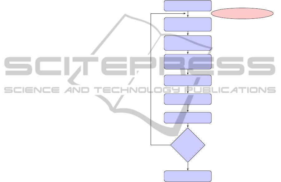
The following figure shows the flow chart of our
proposed algorithm.
Initialize Particles
New Observations
Particles
Generations
Update Particles
Using UKF
Update Particles
Using IEKF
Normalize
Resampling
Output Estimations
More Ob-
servations
Output
yes
no
Figure 1: The schematic description of the proposed
algrithm (HIKPF).
HIKPF Algorithm Steps
—————————————————
Step 1.Initialization: k = 0
FOR i = 1, ....., N
p
Draw the particles x
i
0
from the prior P(x
0
) and set:
¯x
i
0
= E(x
i
0
)
P
i
0
= E[(x
i
0
− ¯x
i
0
)(x
i
0
− ¯x
i
0
)
T
]
¯x
i
0,a
= E[(x
i
0,a
)] = [(x
i
0
)
T
, 0, 0]
T
P
i
0,a
= E[(x
i
0,a
− ¯x
i
0,a
)(x
i
0,a
− ¯x
i
0,a
)
T
] = diag(P
i
0
QR)
END FOR
Step 2. FOR k = 1, 2, ...
(1)FOR i = 1, ....., N
p
VISAPP2013-InternationalConferenceonComputerVisionTheoryandApplications
378

(a) Update the particles using the UKF
Calculate the sigma points
χ
i
k−1,a
= [ ¯x
i
k−1,a
¯x
i
k−1,a
±
q
(n
a
+ λ)P
i
k−1,a
]
Propagate samples into future and compute
the one-step-ahead estimates:
χ
i
k|k−1,x
= f(χ
i
k−1,x
, χ
i
k−1,v
)
Y
i
k|k−1,u f
= h(χ
i
k|k−1,x
, χ
i
k−1,u
)
¯x
i
k|k−1,u f
=
2n
a
∑
j=0
W
( j)
m
χ
( j)i
k|k−1,x
P
i
k|k−1,u f
=
2n
a
∑
j=0
W
( j)
c
[χ
( j)i
k|k−1,x
− ¯x
i
k|k−1,u f
][χ
( j)i
k|k−1,x
−
¯x
i
k|k−1,u f
]
T
¯y
i
k|k−1,u f
=
∑
2n
a
j=0
W
( j)
m
Y
( j)i
k|k−1,u f
Incorporate the new observation y
k
, and update
the one-step-ahead estimates to obtain ¯x
i
k,uf
P
y
k
y
k
=
2n
a
∑
j=0
W
( j)
c
[Y
( j)i
k|k−1,u f
− ¯y
i
k|k−1,u f
][Y
( j)i
k|k−1,u f
− ¯y
i
k|k−1,u f
]
T
P
x
k
y
k
=
2n
a
∑
j=0
W
( j)
c
[χ
( j)i
k|k−1
− ¯x
i
k|k−1,u f
][Y
( j)i
k|k−1,u f
− ¯y
i
k|k−1,u f
]
T
K
k,uf
= P
x
k
y
k
P
−1
y
k
y
k
¯x
i
k,uf
= ¯x
i
k|k−1,u f
+ K
k,uf
(y
k
− ¯y
i
k|k−1,u f
)
P
i
k,uf
= P
i
k|k−1,u f
− K
k,uf
P
y
k
y
k
K
T
k,uf
(b) Use the IEKF to update estimations obtained
through UKF update process
FOR i = 1, ....., N
p
Compute the Jacobians F
i
k
&G
i
k
of the process
model
Update the particles with the IEKF
¯x
i
k|k−1,ie f
= f( ¯x
i
k,uf
)
P
i
k|k−1,ie f
= F
i
k
P
i
k,uf
(F
i
k
)
T
+ G
i
k
FOR j = 1 : c (c is the number of iteration)
Compute the Jacobians H
i
k
j
&U
i
k
j
of the
measurement model
Update the covariance and the state estimate
from the following equations obtained
from IEKF respectively .
K
k
j
,ief
= P
i
k
j
|k
j
−1,ief
(H
i
k
j
)[U
i
k
j
R
k
j
(U
i
k
j
)
T
+
H
i
k
j
P
i
k
j
|k
j
−1,ief
(H
i
k
j
)
T
]
−1
P
i
k
j
,ief
= P
i
k
j
|k
j
−1,ief
− K
k
j
,ief
H
i
k
j
P
i
k
j
|k
j
−1,ief
¯x
i
k
j
,ief
= ¯x
i
k
j
|k
j
−1,ief
+ K
k
j
,ief
(y
k
j
− h( ¯x
i
k
j
,ief
))
let ¯x
i
k
j
= ¯x
i
k
j
,ief
,
ˆ
P
i
k
j
= P
i
k
j
,ief
END FOR
Draw x
i
k
∼ q(x
i
k
|x
i
k−1
, z
k
) = N( ¯x
i
k
j
,
ˆ
P
i
k
j
)
Assign the particle a weight, w
i
k
, according to the
equation below obtained from PF
w
i
k
∝ w
i
k−1
P(z
k
|x
i
k
)P(x
i
k
|P(x
i
k−1
)
q(x
i
k
|x
i
k−1
,z
k
)
END FOR
(2) Normalize the weights
FOR i = 1, ...., N
w
i
k
=
w
i
k
∑
j=1:N
w
i
k
.
END FOR.
(3) Resample
(4) Output: calculate the required estimations
using the particle set.
END FOR.
Step 3. k = k+ 1, go to Step2 or end the algorithm
———————————————————–
4 SIMULATION AND
EXPERIMENTAL RESULTS
The simulation results of the HIKPF algorithm is
presented and discussed in this section as well as
the comparison between HIKPF and the previously
proposed algorithms including PF, PF-EKF, PF-UPF
and PF-IEKF . The system models were taken from
(R Van der Merwe, 2000) as following.
x
k
= 1 + sin(0.4πk) + 0.5x
k−1
+ v
k−1
y
k
=
0.2x
2
k
+ e
k
, if k ≤ 30
0.5x
k
− 2+ e
k
, if k > 30
Where v
k
is a Gamma ς
a
(3, 2) random variable
modelling the process noise, and the measurement
noise u
k
is drawn from a Gaussian distribution
N(0, 0.00001). In this experiment 200 particles are
used and the program is repeated 100 times for time-
steps k = 1, .., 60. The unscented transformation pa-
rameters are set to be α = 1, β = 0, and κ = 2. The
HybridIteratedKalmanParticleFilterforObjectTrackingProblems
379
output of the algorithm is the mean of samples set that
can be computed ˆx =
1
N
∑
N
s
j=1
x
j
t
. The mean square er-
rors of each run is defined as
MSE =
1
T
T
∑
k=1
( ˆx
k
− x
k
)
!
1
2
(11)
Figure 2 Shows the true and the estimated state of the
system HIKPF and the other methods. It is clear from
the figure that particle filter (PF) and extended kalman
particle filter ( PF-EKF) deviate from the true states
at some time steps. The unscented Kalman particle
filter(PF-UKF) and iterated extended kalman particle
filter (PF-IEKF) gives better performance than PF and
PF-EKF but less than our proposed system (HIKPF).
5 10 15 20 25 30 35 40 45 50 55 60
−2
0
2
4
6
8
10
12
14
Time
Estimated states and true states
True x
PF
PF−EKF
PF−UKF
PF−IEKF
HIKPF
Figure 2: Estimation of the system state generated by dif-
ferent particles filters.
The performance evaluation of our system com-
pared with other methods is shown in table 1. In
this table, our proposed system (HIKPF) gives the
best performance with the lowest mean and variance
with mean value 0.015607 and variance value (
Var
)
0.00000395.
Table 1: Estimation of means and variances of
MSE
of dif-
ferent particles filters over 100 independent runs.
Algorithm
MSE
mean Var
PF 0.25881 0.057151
PF-EKF 0.32392 0.021656
PF-UKF 0.077684 0.006589
PF-IEKF 0.049368 0.0015238
HIKPF 0.015607 0.00000395
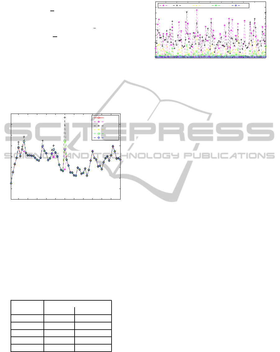
Estimation of mean squars errors (
MSEs
) of differ-
ent particle filters are shown in Figure 3 In this fig-
ure, it is clear that the bottom real line (Blue Line) is
the HIKPF performance line. The proposed algorithm
10 20 30 40 50 60 70 80 90 100
0
0.1
0.2
0.3
0.4
0.5
0.6
0.7
0.8
0.9
1
Run(s)
MSE
PF PF−EKF PF−UKF PF−IEKF HIKPF
Figure 3:
MSEs
estimation of different particles filters at
each run.
give the lowest mean square error at every indepen-
dent run.
5 CONCLUSIONS
A new algorithm referred to as the hybrid iterated
Kalman particle filter (HIKPF) is proposed. The pro-
posed algorithm is developed from unscented Kalman
filter (UKF) and iterated extended Kalman filter
(IEKF) to generate the proposal distribution leading
to efficientuse of the latest observations and generates
more close approximation of the posterior probability
density. Numerical simulation and experiment results
show that HIKPF algorithm is much robust than the
previously proposed algorithms such as (PF, PF-EKF,
PF-UPF and PF-IEKF).
REFERENCES
Arulampalam, M., Maskell, S., Gordon, N., and Clapp,
T. (2002). A tutorial on particle filters for online
nonlinear/non-gaussian bayesian tracking. In IEEE
Transactions on Signal Processing. IEEE Signal Pro-
cessing Society,Vol. 50, pp. 174-188.
Broida, T. and Chellappa, R. (1986). Estimation of object
motion parameters from noisy images. In IEEE Trans-
actions on Pattern Analysis and Machine Intelligence.
IEEE Computer Society Washington, DC, USA,Vol.
8, No. 1, pp. 90-99.
Collins, R., Lipton, A., Kanade, T., Fujiyoshi, H., Duggins,
D., Tsin, Y., Tolliver, D., Enomoto, N., and Hasegawa,
O. (2000). System for video surveillance and monitor-
ing. In Technical Report CMU-RI-TR-00-12. Robitics
institute.
Fen, X. and Ming., G.(2010). Pedestrian tracking using par-
ticle filter algorithm. In International Conference on
Electrical and Control Engineering. IEEE Computer
Society Washington, DC, USA,pp.1478-1481.
Gelb, A. (1974). Applied Optimal Estimation. M.I.T. Press,
Cambridge, 1st edition.
Gordon, N., Salmond, D., and Smith, A. (1993). Novel
approach to nonlinear/non-gaussian bayesian state es-
VISAPP2013-InternationalConferenceonComputerVisionTheoryandApplications
380

timation. In IEEF Proceedings Radar and Signal Pro-
cessing. IET,Vol. 1, pp. 107-113.
Isard, M. and Blake, A. (1998). Condensation conditional
density propagation for visual tracking. In Interna-
tional Journal of Computer Vision. Kluwer Academic
Publishers Hingham,MA,USA, Vol. 29, No. 1, pp. 5-
28.
Julier, S. (2002). The scaled unscented transformation. In
Proceedings of the 2002 American Control Confer-
ence2. IEEE Conference Publications,Vol 6,PP.4555-
4559.
Julier, S., Jeffrey, J., and Uhlmann, K. (2002). Reduced
sigma point filters for the propagation of means and
covariances through nonlinear transformations. In
In Proceedings of the American Control Conference.
IEEE Conference Publications Vol 2, pp. 887-892.
Julier, S. J. and Uhlmann, J. K. (2004). Unscented filtering
and nonlinear estimation. In Proceedings of the IEEE.
IEEE,Vol 92, pp. 401-422.
kyung-min Cho, jeong-hun Jang, and ki-sang Hong (2001).
Adaptive skin-color filter. In Pattern Recognition. El-
sevier, Vol 34,pp. 1067-1073.
Lefebvre, T. and Bruyninckx, H. (2004). Kalman filters for
nonlinear systems: A comparison of performance. In
International Journal of Control. Vol 77,pp.639-653.
Liang-qun, L., Hong-bing, J., and Jun-hui, L. (2005).
The iterated extended kalman particle filter. In Pro-
ceedings International Symposium on Communication
and Information Technologies 2005. IEEE Conference
Publications,Vol 2,pp.1213-1216.
Lipton, A., Fujiyoshi, H., and Patil, R. (1998). Moving tar-
get classification and tracking from real-time video. In
Proceeding of IEEE Workshop Applications of Com-
puter Vision. IEEE Conference Publicationsn,pp. 8-
14.
LIU, Y., Haizho, A., and Guangyou, X. (2001). Moving ob-
ject detection and tracking based on background sub-
traction. In Proceeding of Society of Photo-Optical
Instrument Engineers. Vol. 4554, pp. 62-66.
McIvor, A. M. (2000). Background subtraction tech-
niques. In Proceeding of Image and Vision Comput-
ing. IVCNZ00, Hamilton, New Zealand.
Meyer, D., Denzler, J., and Niemann, H. (1998). Model
based extraction of articulated objects in image se-
quences for gait analysis. In Proceeding of IEEE Int.
Conf. Image Proccessing. IEEE Conference Publica-
tions,Vol 3,pp.78-81.
Phung, S., Chai, D., and Bouzerdoum, A. (2003). Adap-
tive skin segmentation in color images. In Proceed-
ing of IEEE International Conference on Acoustics,
Speech and Signal Processing. IEEE Conference Pub-
lications,Vol. 3, pp. 353-356.
R Van der Merwe, A. D. (2000). The unscented particle
filter. In Advances in Neural Information Processing
Systems.
Rawlings, J. and Bakshi, B. (2006). Particle filtering and
moving horizon estimation. In Computers and Chem-
ical Engineering. Elsevier,Vol 30,pp. 1529-1541.
Ristic, B., Arulampalam, S., and Gordon, N. (2004). Be-
yond the Kalman filter: Particle filters for tracking
applications. Artech House.
Soderstorm, T. (2002). Discrete-time stochastic systems,
in: Advanced Textbooks in Control and Signal Pro-
cessing. Springer.
Sugandi, B., Kim, H., Tan, J. K., and Ishikawa, S. (2009).
A moving object tracking based on color information
employing a particle filter algorithm. In Artificial Life
and Robotics. Springer Japan,Vol 14,pp. 39-42.
Wan, E. and van der Merwe, R. (2001). Chapter 7: The un-
scented kalman filter,. In Kalman Filteringand Neural
Networks, S. Haykin, Ed.,. Wiley Publishing.
Zhiqiang, W., Peng, Z., Deng, X., and Li.Shifeng (2011).
Particle filter object tracking based on multiple cues
fusion. In Advanced in Control Engineering and In-
formation Science. Procedia Engineering,Vol 15, pp.
1461-1465.
Zhonga, Q., Qingqinga, Z., and Tengfeia, G. (2012). Mov-
ing object tracking based on codebook and parti-
cle filter. In International Workshop on Informa-
tion and Electronics Engineering. Procedia Engineer-
ing,Vol 29,pp. 174-178.
HybridIteratedKalmanParticleFilterforObjectTrackingProblems
381
