
Detecting Focal Regions using Superpixels
Richard Lowe and Mark Nixon
CSPC Group, University of Southampton, Burgess Rd, Southampton, U.K.
Keywords:
Superpixel, Focus Region, Light Field.
Abstract:
We introduce a new method that can automatically determine regions of focus within an image. The focus
is determined by generating Content-Driven Superpixels and subsequently exploiting consistency properties
of scale-space. These superpixels can be analysed to produce the focal image regions. In our new analysis,
Light-Field Photography provides an efficient method to test our algorithm in a controlled manner. An image
taken with a light-field camera can be viewed from different perspectives and focal planes, and so by manually
modifying the focal plane we can determine if the extracted focal areas are correctly extracted. We show
improved results of our new approach compared with some prior techniques and demonstrate the advantages
that our new approach can accrue.
1 INTRODUCTION
The ability to focus is implicit in image formation. In
photography, there are passive and active approaches
to achieve image autofocus wherein the image clar-
ity depends on optical parameters. Passive autofocus
approaches analyse local image contrast as part of a
feedback mechanism driving the lens motor whereas
active approaches aim to sense distance to derive fo-
cus capability. As such, we can enjoy clear pho-
tographs which can usually be acquired with the ob-
ject of interest in sharp focus.
In contrast to the plethora of approaches for im-
age autofocus, there are few approaches which can be
applied to analyse an image to determine the regions
which are in sharp focus. One such approach, the Sum
Modified Laplacian (Nayar and Nakagawa, 1994),
was designed to analyse shape from focus using the
relative differences in contrast at differing image res-
olutions. More recent works are concerned with the
extraction of edge information (Tai and Brown, 2009)
as the edges contain more high frequency informa-
tion. Another method uses Gabor wavelets (Chen and
Bovik, 2009) that are tuned to detect high frequency
image components. Other methods (Liu et al., 2008;
Kovacs and Sziranyi, 2007; Levin, 2007) attempt to
model a blur kernel and use convolution to inverse
the blurring process. These algorithms are actually
de-blurring algorithms and have a different intention
(to remove blurring) but operate in a similar way.
The method we choose to compare with is the
Sum Modified Laplacian as it is well-established. We
also compare with approaches described in (Levin,
2007) and (Liu et al., 2008), though these methods
require the tuning of several parameters. They also
rely on feedback from human vision to determine if
the result is ‘correct’. As these rely on sharpness of
edge information, they are also sensitive to noise.
We introduce a new approach that can be applied
to explicitly extract focal regions of a single image
without choice of parameters. By exploiting the com-
bined properties of the scale-space and superpixels,
it is possible to extract uniform regions in scale and
therefore determine the most likely regions of image
focus.
Superpixels are a way of altering the representa-
tion of an image. They replace the grid of equally
sized pixels with unequal regions that are unique
to each image; aiding the description of image ob-
jects. As superpixels have the property of shape, they
can convey local information about the image. Intu-
itively, this also improves speed of further process-
ing as superpixels significantly reduce the number of
pixels. We use Content-Driven Superpixels (Lowe
and Nixon, 2011) since, unlike many superpixel al-
gorithms, they are designed to produce an unspecified
number of superpixels that are consistent in colour but
not size. Using this in conjunction with a scale-space
representation yields a set of superpixels that are uni-
form with respect to colour across multiple scales.
The distribution of superpixels through scale can be
used to infer where the image has been affected by
smoothing and therefore where the image is in focus
as illustrated in Figure 1.
264
Lowe R. and Nixon M..
Detecting Focal Regions using Superpixels.
DOI: 10.5220/0004212102640270
In Proceedings of the International Conference on Computer Vision Theory and Applications (VISAPP-2013), pages 264-270
ISBN: 978-989-8565-47-1
Copyright
c
2013 SCITEPRESS (Science and Technology Publications, Lda.)
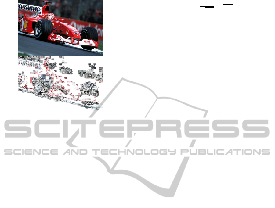
Figure 1: Determining focused areas of an image using su-
perpixels.
With conventional images it is difficult to ascer-
tain, other than with human vision, whether image
focus has been correctly localised. For a principled
analysis of focus detection, we use Light Field Pho-
tography (LFP) to validate our approach as it provides
a controlled environment with which to vary the focal
plane in an image. Our results can show precisely that
as image focus varies, the extracted focus regions of
the image correspond to that change.
The paper is arranged as follows: firstly, scale-
space is introduced. Content-Driven Superpixels are
then described and extended into 3D in order to anal-
yse scale-space. Subsequently, Light Field Photogra-
phy is described as the method with which to generate
the test images to analyse performance. The mecha-
nism of focus detection is then described, followed by
a presentation and discussion of the results.
2 SCALE-SPACE
Developed by Witkin (Witkin, 1983), scale-space is
a one-parameter family of derived images that suc-
cessively smoothes an image, removing more high-
frequency features with each scale. Among other
things, it has been used in detecting scale-invariant
edges (Bergholm, 1987), as a basis for the popular
SIFT and SURF operators, and also saliency (Kadir
and Brady, 2001). Edges are deemed to be more
significant if they persist for several scales whereas
saliency is more significant if it persists over few
scales. To generate the scale-space, the new images
need to be derived by convolving the image with a
Gaussian filter, given in Equation 1, where t denotes
the scale.
g(x, y, t) =
1
√
2πt
e
(−
x
2
+y
2
2t
)
(1)
The choice of t is based on a logarithmic sam-
pling. To efficiently construct the scale-space, t is
chosen such that the difference between scales is
maximised without losing detail. Equation 2 pro-
vides a method of selecting t (Lindeberg, 1994). τ
is the transformation of the image as a function of
the smoothing parameter t and A is a free parame-
ter. This motives the choice of sampling to be t =
{1, 4, 16, 64, 256}, the use of which causes the loga-
rithmic sampling to produce a linear increase in value
for A and therefore a linear difference between scales.
τ(t) = A logt (2)
The scale-space is then collapsed into a single vol-
ume, successive two-dimensional slices represent in-
creasing levels of detail.
We can infer from the scale-space that if a spatial
region is consistent over all scales then smoothing has
had little effect. Therefore this region contains little
high frequency information and is more likely to be
out of focus.
3 CONTENT-DRIVEN
SUPERPIXELS
Content-Driven Superpixels (CDS) (Lowe and Nixon,
2011) is a new approach designed to allow superpixel
coverage to express the underlying structure of an im-
age. An image will contain as many superpixels as
needed and is not controlled by initialisation param-
eters. As such, it is an appropriate way of exploring
how the scale-space changes with increased smooth-
ing, without imposing supervised initialisation.
The CDS approach is designed to grow superpixel
regions, splitting them as they become more complex
in order to retain colour uniformity. Extending this
to consider the scale-space means that the superpixels
will represent uniform colour in scale and in space.
The distribution will describe the underlying structure
of the scale-space and this information can be anal-
ysed to determine the focal regions. These superpix-
els shall be referred to as supervoxels as they occupy
a third dimension, despite the fact that this third di-
mension is not spatial.
3.1 Extending the Algorithm to 3D
Fortunately, as CDS is a combination of standard
spatial computer vision techniques, each sub-process
can be separately transposed into 3D. The two main
DetectingFocalRegionsusingSuperpixels
265

mechanisms: ‘Distance Transform’ and ‘Active Con-
tours without Edges’ are ideally suited for 3D.
3.1.1 Distance Transform
Supervoxel growth is achieved using a distance trans-
form of every supervoxel. This transforms each su-
pervoxel S such that a set of voxels at locations i, j, k
within the supervoxel display the distance D to the
background (in this case, the region in which super-
voxels have yet to form). Supervoxel edges therefore
have a distance of one from the background. A binary
volume V is used to calculate the distance transform
where True denotes that a supervoxel covers this point
in the volume and False otherwise. The background
is therefore all the False points. The same volume is
used to individually grow each supervoxel.
The Distance Transform in 3D transforms a vol-
ume such that the volume displays the distance D
of each voxel at location (i, j, k)to the nearest back-
ground location (x, y, z). This is given in Equation 3.
D = min
x,y,z: V (x,y,z)=False
q
(i −x)
2
+ ( j −y)
2
+ (k −z)
2
(3)
This growth occurs at each iteration t. The growth
of the supervoxel S is given in Equation 4.
S
<t+1>
= S
<t>
∪{(x, y, z) : D(x, y, z) = 1} (4)
3.1.2 Active Contours without Edges
Active Contours Without Edges (ACWE) (Chan and
Vese, 2001; Chan et al., 2000) aims to partition an im-
age into two regions of constant intensities of distinct
values. These values form the positive and negative
parts of a signed distance function, Ω
D
. Equation 5
describes the force F that iteratively updates the dis-
tance function. For example F is large and negative
for a particular pixel if it is currently labelled as pos-
itive and is distinct from the mean of the region that
it is contained in. F is small for a pixel if it is similar
to the mean of the region it is contained in. By iter-
atively updating the distance function of each pixel,
the boundary between the positive and negative re-
gions moves. Each voxel therefore becomes part of
the region it best matches.
The new supervoxels, C
u
,C
v
, are taken to be the
positive and negative parts of the newly formed dis-
tance function, Ω
0
D
. To use this algorithm with super-
voxels it is necessary to define Ω(x, y, z) as a vector
that contains a set of all the voxels within the super-
voxel.
F(x, y, z) =
Z
Ω
1
N
N
∑
i=1
|I
i
(x, y, z) −u
i
|
2
dxdydz
−
Z
Ω
1
N
N
∑
i=1
|I
i
(x, y, z) −v
i
|
2
dxdydz
(5)
The segmentation criterion of either region u, v is
given as the average of the means (u
i
, v
i
) of each of
the N colour channels V
i
of the volume V ; shown in
Equation 6. Supervoxel division occurs if there is a
significant difference between any of the colour chan-
nels.
u
i
=
R
Ω
V
i
(x, y, z)dxdydz
R
Ω
Ω(x, y, z)dxdydz
, ∀Ω
D
(x, y, z) > 0 (6)
v
i
=
R
Ω
V
i
(x, y, z)dxdydz
R
Ω
Ω(x, y, z)dxdydz
, ∀Ω
D
(x, y, z) ≤ 0
ACWE still requires the separation of a supervoxel
into two regions u, v, but these regions now occupy
a 3D signed distance function Ω
D
(x, y, z). The two
regions C
u
,C
v
are given in Equation 7.
C
u
= {(x, y, z) : Ω
0
D
(x, y, z) > 0} (7)
C
v
= {(x, y, z) : Ω
0
D
(x, y, z) ≤ 0}
3.2 Applying CDS to Focus Detection
Firstly, images are converted into a set of 3D scale-
space representations using the values of t defined in
Section 2. By using scale-space for superpixels, the
aim is to produce superpixels that have context over
scale; scale-persistent superpixels are more likely to
be stable whereas scale-varying superpixels are more
likely to be in feature-rich areas of the image.
By grouping regions of scale-space, it is possible
to gain information about the nature of that region of
the image. The idea is that superpixels that exist in
the low detail area of the scale-space are less likely to
contribute the high-frequency content present in the
focused region of the original volume. A set of super-
voxels is initialised in the least-detailed layer of the
scale-space. This is done such that as the supervoxels
grow through more complex layers of the space, they
increase in number. Initialising in the most complex
layer would require more supervoxels than necessary
to represent the least complex layer.
To reveal the parts of the image, as the volume
being analysed is smoothed, the most smoothed layer
will contain the least information. The focus is de-
termined as the lowest detail layer t
min
in which the
supervoxel still exists. Therefore the supervoxels that
exist in the first layer have the lowest focus value. Su-
pervoxels that exist solely in the highest layer have
VISAPP2013-InternationalConferenceonComputerVisionTheoryandApplications
266
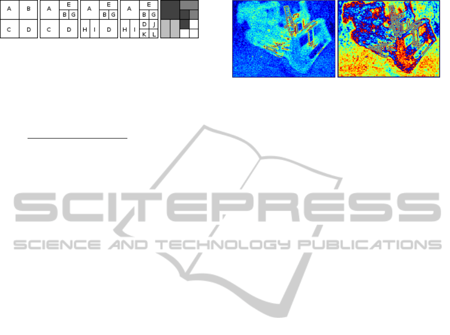
(a) t = 0 (b) t = 1 (c) t = 2 (d) t = 3 (e) Result
Figure 2: Illustrating how focus is determined.
the maximum focus value. This is shown in Equa-
tion 8. The focus measure F for a supervoxel s is
controlled by the first layer t in which that supervoxel
exists. T
max
is the number of layers in the image.
F(s) =
1
T
max
−min{t : s(x, y,t) > 0}
;(x, y) ∈I, 0 ≤t < T
max
(8)
A hypothetical example is given in Figure 2,
which shows four layers of the same volume, where
each labelled region represents a supervoxel. Multiple
layers can contain the same supervoxel, for example
region A which exists for all layers, but the minimum
layer is t = 0. Each subfigure is given with the layer
t in the volume it represents. Figure 2(d) shows the
least smoothed layer, ie. the original image.
As region A remains constant, no change in space
or scale has been detected and can be considered out
of focus. Regions A,B,C,D are therefore given a focus
value of F(s) = 0.25. Next E,G have a focus of 0.5
as they first exist in layer t = 1, and regions H,I have
a focus value of 0.75. Regions J,K,L are therefore the
most likely to be in focus, with F(s) = 1. Figure 2(e)
shows this graphically, where brightness indicates a
higher focus value. Each location in space shows the
highest focus value at that point. For example in the
case of regions C,H,I, even though they occupy the
same spatial location, the focus values of H and I are
given as the result as they have the higher focus value.
4 SUM MODIFIED LAPLACIAN
As a comparative approach, an established method
of analysing focus is the Sum Modified Laplacian
(SML). The focus is derived from the image I at levels
spaced by a step ∆s.
ML(x, y) = |2I(x, y) −I(x −∆s, y) −I(x + ∆s, y)|
+|2I(x, y) −I(x, y −∆s) −I(x, y + ∆s)| (9)
The focus measure (Equation 10) at (i, j) is evalu-
ated as the neighbourhood (of size N) sum of the mod-
ified Laplacian (Equation 9) which exceed a threshold
T . The step size can be varied to locate different tex-
ture sizes.
F(i, j) =
i+N
∑
x=i−N
j+N
∑
y= j−N
ML(x, y)|ML(x, y) ≥ T (10)
(a) N = 2 (b) N = 4
Figure 3: Showing the same image using different values
for N in SML. The red areas depict distinctly different areas
of focus in each image.
This is problematic as it will only select textures
of a chosen size and will be affected by the size of the
neighbourhood. This makes using the algorithm as a
focus measure subject to human opinion and insight.
The results of focus detection in Figure 3 show that
the quality of the result relies on selection of appro-
priate parameter values, and the selection of those pa-
rameters relies on human visual analysis. This prop-
erty is not a problem if one is comparing images gen-
erated using the same parameters.
In contrast, our new approach can inherently lo-
cate scale-varying regions without parameterisation
or supervision. CDS also is region based, thereby se-
lecting regions of interest which is more useful than
individual pixels.
5 GENERATING THE TEST
IMAGES
Light Field Photography (LFP)(Levoy and Hanrahan,
1996) is continuing to gather interest. LFP is cur-
rently achieved (Wilburn et al., 2005) using either an
array of cameras or a single camera moved through
a 2D array. A capture method using a single expo-
sure (Ng et al., 2005; Adelson and Wang, 1992) is
now being developed commercially. By considering
an image as a 2D slice of a 4D function, new views
of the same scene can be obtained by extracting dif-
ferent slices. This is exploited in several ways, the
relevant one in this case being the ability to refocus a
light-field after it has been taken.
We use this ability is used to generate controlled
test images. This allows a principled analysis of fo-
cus, this being the first time such a test procedure has
been achieved. A series of images are chosen from
a light-field that focus on a different section of the
scene, thereby allowing the efficacy of focus detec-
tion to be measured. An example series of images is
given in Figure 4 which shows ability of LFP to focus
on foreground and background objects.
DetectingFocalRegionsusingSuperpixels
267
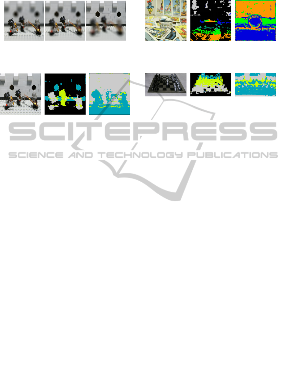
(a) near (b) middle (c) far
Figure 4: Illustrating the effect of change of focus on a light-
field.
(a) Reference image (b) The labelled focus
response of each image
(c) The labelled SML
response of each image
Figure 5: Result on the lego image.
6 RESULTS
6.1 Light-field Experiments
We evaluate our algorithm using the controlled im-
ages derived from light fields. There are two ways of
analysing the quality of the results. Firstly, the ‘fo-
cus response’, where the supervoxels are drawn on
the image as an alpha layer to show which parts are
in focus. This response is then used in conjunction
with the depth information of the light field to deter-
mine which depths of the image are extracted as ‘in
focus’. This can then be used to label the image with
the corresponding depths. The images in this section
are taken from light-field images available through the
Stanford Computer Graphics Laboratory
1
. All SML
images are generated using T = 1 and ∆S = 1 which
retains the highest proportion of high-frequency in-
formation.
Figure 5 shows the result on the lego image in Fig-
ure 4. Figure 5(a) shows the image totally in focus for
reference. Figure 5(b) shows the focus of each image
as the focal depth changes. The coloured labels corre-
spond to the focus of different images, and so here the
change in focus through the image can be observed by
areas of the image being occupied by distinct bands of
colour. Grey corresponds to image 0, green to image
1 and blue to image 2. Black regions were not la-
belled as in focus in any image. CDS clearly shows
the change in focus in the image, whereas SML in-
1
http://lightfield.stanford.edu/
(a) Reference image (b) The labelled focus
response of each image
(c) The labelled SML
response of each image
Figure 6: Result on the image containing tarot cards.
(a) Reference image (b) The labelled focus
response of each image
(c) The labelled SML
response of each image
Figure 7: Result for the chess image.
correctly misses the central figure and mis-labels the
background.
Figure 6 shows the response to a light-field image
containing tarot cards. The CDS response is shown
in Figure 6(b) where the objects at each depth belong
to different image labels when the object was in fo-
cus. Orange corresponds to image 0; green to image
1; cyan to image 2; blue to image 3 and grey to image
4. Here, the SML response shows no clear distinction
between the images, and the bands present in the CDS
response are missing. There is also significantly more
noise, as most of the pixels are labelled as being in
focus, whereas CDS shows clear regions of no focus
at all.
The image in Figure 7 again shows a clear tran-
sition from foreground to background as the focus of
the image changes. In the CDS response there is once
again a clear separation of each response, SML can-
not correctly distinguish the focus as the focal depth
changes. CDS can determine which parts of the im-
age is background whereas SML cannot.
6.2 Image Experiments
Figure 8 compares the result from CDS with three
other techniques. The brightness of the result denotes
how focused that area is. It is difficult to compare
with other approaches as only the classification result
is available and their techniques are not yet evaluated
using LFP. However, we detect largely the same re-
gions as both. There is some inclusion of the back-
ground, however this is at a lower focus value to the
cyclist. The CDS approach requires no tuning which
is implicit in all other techniques. CDS clearly detects
the focused cyclist well.
The algorithm has also been applied to several
VISAPP2013-InternationalConferenceonComputerVisionTheoryandApplications
268
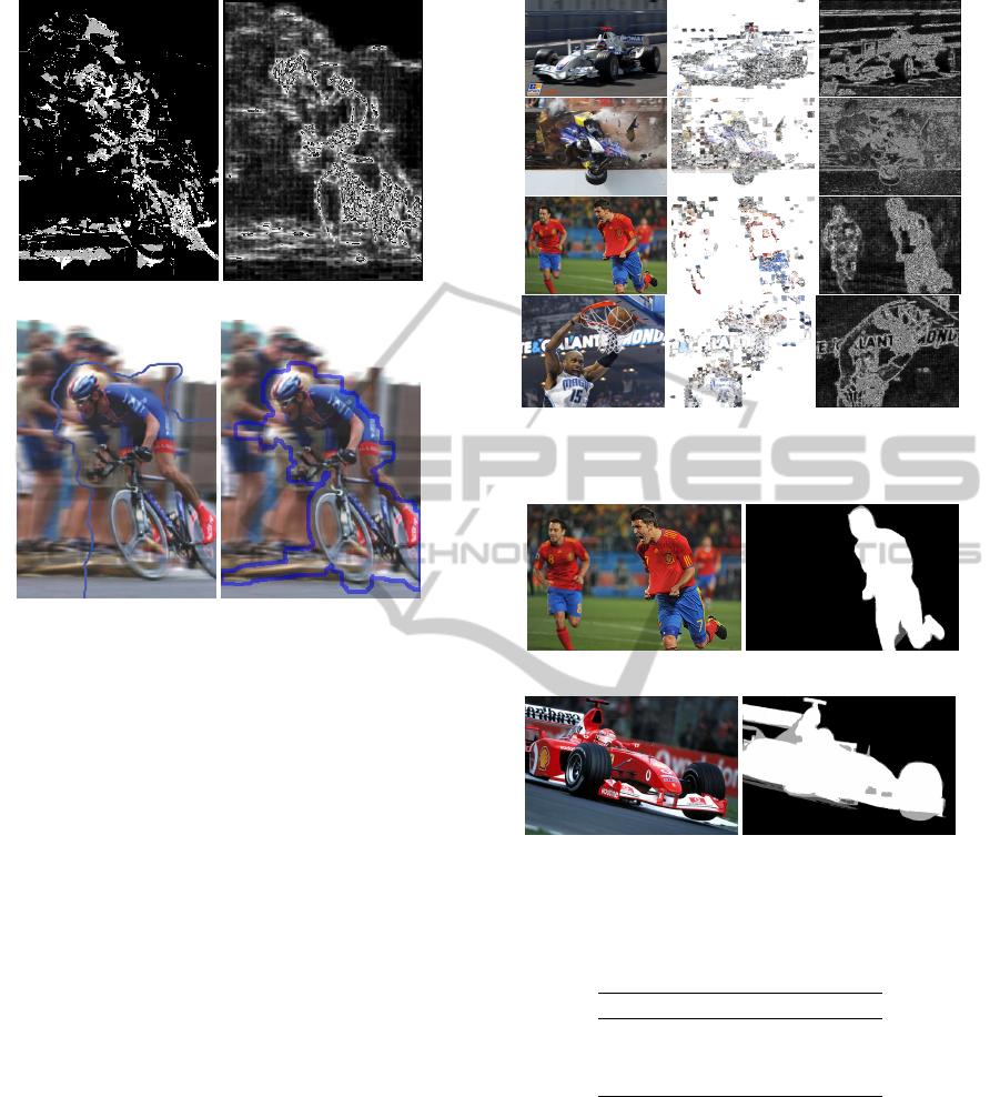
(a) CDS (b) SML
(c) Levin (Levin, 2007) (d) Liu (Liu et al., 2008)
Figure 8: Comparing CDS with other techniques.
sports images shown in Figure 9. Motorsport images
are particularly suited to illustrating the ability to ex-
tract focused regions since the images produced con-
tain large amounts of motion blur. Note that neither
technique extracts regions of uniform colour. This is
because, inherently, contrast does not change in uni-
form regions.
There are notable differences between CDS and
SML. Firstly, SML does a much better job of extract-
ing the basketball image. However in the car images,
SML detects areas of erroneous focus in the back-
ground that are attributed to strong edge information.
As CDS does not rely on edge information to detect
focus, these regions are not detected in our new ap-
proach.
Table 1 compares the two images in Figure 10 for
both SML and CDS by calculating the fraction of the
output that is contained within the ground truth. The
ground truth was derived by averaging the response
of five different human ‘labelers’. The ‘labelers’ were
instructed to highlight the regions of the image which
appeared to be in sharp focus. This implies that some
uniform areas are manually labelled to be in sharp fo-
cus whereas these areas are detected by neither SML
nor CDS. It shows that while SML can sometimes
have a better response, it is highly dependent on the
input parameters to the algorithm; the results can vary
(a) Original (b) CDS (c) SML
Figure 9: Sports images.
(a) Football image (b) Ground truth
(c) Car image (d) Ground truth
Figure 10: Test images used to compare SML and CDS.
Table 1: Results on two images to show the percentage of
the response that corresponds with a ground truth.
Technique Football Car
CDS 0.49 0.60
SML Min 0.21 0.40
SML Max 0.43 0.74
by as much as 50%. CDS performs as well as the best
SML result without supervision or manual interven-
tion. An analysis by human ‘labelers’ also introduces
some confusion as in the football image one player is
not labelled however it is detected by both algorithms
as shown in Figure 9.
DetectingFocalRegionsusingSuperpixels
269

7 DISCUSSION
Any image can contain both focused and unfocused
regions. There is no way to test the validity of a focus
detection algorithm without a reliable metric which
can quantify focus accuracy. By using the depth in-
formation from the light field we have shown that it is
possible to show that the focal response corresponds
to a specific image depth and that this depth changes
consistently with image focus.
Essentially, CDS highlights the parts of the image
that are in focus but also are more likely to contain
high-frequency information. As CDS creates new su-
perpixels on detecting image variation, there will be
some constant colour areas of the image that do not
change significantly with blurring. The result will be
that these regions are not marked as in focus. While
other methods can extract points of focus within the
image, these methods rely on tuning of the algorithm
parameters. As we have shown, the results on SML
can vary by as much as 50% depending on the se-
lection of adequate parameters. In addition, as these
are edge based techniques, they also rely on the ab-
sence of noisy edges in the image. CDS negates this
by considering regions within the image, as there is
an inherent averaging within ACWE.
This paper has described the first application of
superpixels in conjunction with scale-space. Apply-
ing CDS to the task of focus detection gives a result
which has been shown to correspond accurately to the
focal regions of the image. Crucially, it is unsuper-
vised and as such gives an unbiased representation of
the focus within an image, which can be demonstrated
by using the unique properties of Light Field Photog-
raphy.
REFERENCES
Adelson, E. H. and Wang, J. Y. A. (1992). Single lens
stereo with a plenoptic camera. IEEE Transactions on
Pattern Analysis and Machine Intelligence, 14(2):99–
106.
Bergholm, F. (1987). Edge Focusing. IEEE TPAMI,
9(6):726–741.
Chan, T., Sandberg, B., and Vese, L. (2000). Active
Contours without Edges for Vector-Valued Images.
Visual Communication and Image Representation,
11(2):130.
Chan, T. F. and Vese, L. A. (2001). Active Contours Without
Edges. IEEE Trans. Image Processing, 10(2).
Chen, M.-J. and Bovik, A. C. (2009). No-reference image
blur assessment using multiscale gradient. In Quality
of Multimedia Experience, 2009. QoMEx 2009. Inter-
national Workshop on, pages 70–74.
Kadir, T. and Brady, M. (2001). Saliency, Scale and Image
Description. IJCV, 45(2):83–105.
Kovacs, L. and Sziranyi, T. (2007). Focus area extraction
by blind deconvolution for defining regions of inter-
est. Pattern Analysis and Machine Intelligence, IEEE
Transactions on, 29(6):1080–1085.
Levin, A. (2007). Blind motion deblurring using image
statistics. Advances in Neural Information Processing
Systems, 19:841.
Levoy, M. and Hanrahan, P. (1996). Light field rendering.
In Proc. Conf. on Computer Graphics and Interactive
Techniques, pages 31–42.
Lindeberg, T. (1994). Scale-space theory: A basic tool for
analyzing structures at different scales. Journal of Ap-
plied Statistics, 21(1):225–270.
Liu, R., Li, Z., and Jia, J. (2008). Image partial blur de-
tection and classification. In Computer Vision and
Pattern Recognition, 2008. CVPR 2008. IEEE Con-
ference on, pages 1–8.
Lowe, R. and Nixon, M. (2011). Evolving Content-Driven
Superpixels for Accurate Image Representation. In
Proc. ISVC2011, volume 6938 of Lecture Notes in
Computer Science, pages 192–201. Springer-Verlag.
Nayar, S. K. and Nakagawa, Y. (1994). Shape from fo-
cus. Pattern Analysis and Machine Intelligence, IEEE
Transactions on, 16(8):824–831.
Ng, R., Levoy, M., Br
´
edif, M., Duval, G., Horowitz, M., and
Hanrahan, P. (2005). Light field photography with a
hand-held plenoptic camera. Computer Science Tech-
nical Report CSTR, 2.
Tai, Y.-W. and Brown, M. S. (2009). Single image defo-
cus map estimation using local contrast prior. In Im-
age Processing (ICIP), 2009 16th IEEE International
Conference on, pages 1797–1800.
Wilburn, B., Joshi, N., Vaish, V., Talvala, E. V., Antunez, E.,
Barth, A., Adams, A., Horowitz, M., and Levoy, M.
(2005). High performance imaging using large camera
arrays. ACM Transactions on Graphics, 24(3):765–
776.
Witkin, A. (1983). Scale-space filtering. Intl. Joint Conf.
Art. Intell., 2:1019–1022.
VISAPP2013-InternationalConferenceonComputerVisionTheoryandApplications
270
