
A Prior-knowledge based Casted Shadows Prediction Model Featuring
OpenStreetMap Data
M. Rogez
1,2
, L. Tougne
1
and L. Robinault
1,2
1
Universit
´
e de Lyon, CNRS, Universit
´
e Lyon 2, LIRIS, UMR5205, F-69676, Lyon, France
2
Foxstream, Vaulx en Velin, France
Keywords:
Scene Modeling, Shadows Prediction, OpenStreetMap.
Abstract:
We present a prior-knowledge based shadow prediction model, focused on outdoors scene, which allows to
predict pixels, on the camera, which are likely to be part of shadows casted by surrounded buildings. We
employ a geometrical approach which models surrounding buildings, their shadow and the camera. One in-
novative aspect of our method is to retrieve building datas automatically from OpenStreetMap, a community
project providing free geographic data. We provide both qualitative and quantitative results in two different
contexts to assess performance of our prediction model. While our method cannot achieve pixel precision eas-
ily alone, it opens opportunities for more elaborate shadow detection algorithms and occlusion-aware models.
1 INTRODUCTION
Object detection, recognition and tracking are com-
mon tasks in the video-surveillance field. Methods to
achieve these tasks often rely on segmentation as a
first step to extract relevant segments which can be
further analyzed by computer learning methods for
identification. Depending on the robustness of fea-
tures chosen in the learning step, accurate segmen-
tation might be of prime importance. Indeed under-
segmentation might include pixels with very different
colors which will decrease performance of colorimet-
ric features. Furthermore, shapes features might suf-
fer as well from over- or under-segmentation.
One of the main challenge to address to obtain
accurate segmentation is shadows. Indeed, casted
shadow are often undissociated from the object that
cast them, especially for objects on the ground such
as cars or pedestrians.
Recent shadows detection techniques have been
reviewed by Sanin, Sanderson and Lovell (Sanin
et al., 2012). They classify shadow detection algo-
rithm based on the features used:
Chromaticity-based methods often use a linear
color attenuation model: A shadowed pixel lowers its
intensity (ie gets darker) without changing its chro-
maticity. In this context, it is often desirable to use
a color space, which eases the intensity/chromaticity
separation such as HSV (Cucchiara et al., 2001) or
CIELAB (Lalonde et al., 2009).
Physically-based methods employ physical prop-
erties of light sources and/or physical properties
of material surfaces to achieve shadow detection.
Nadimi and Bhanu (Nadimi and Bhanu, 2004), for
instance, model both contributions of the sun (white
light) and of the sky (blue light) to build their color at-
tenuation model. Huang and Chen (Huang and Chen,
2009) use more general illumination model called Bi
Illuminant Dichromatic Reflection model to detect
shadows. Finlayson, Hordley, Ku and Drew (Fin-
layson et al., 2002) make assumptions on the camera
sensor as well to derive intrinsic image and remove
shadow (Finlayson et al., 2006).
Geometric-based methods infer casted shadows
from the geometric description of objects composing
the current scene. These methods are often tailored
for specific object shadows such as cars (Leotta and
Mundy, 2006) or pedestrians. They often assume that
there is only a single light source and that shadow is
casted on a flat surface.
Texture-based methods assume that texture fea-
tures of a given region are mostly preserved when
shadowed. These methods usually work in two steps:
first, they select shadow pixels candidates (a weak
shadow detector is perfectly suited for this), then, cor-
relate texture of the candidate region in the current
image with the one found in the background model
(Leone and Distante, 2007).
We investigate in this article another way, which
explores the possibility of using contextual knowl-
602
Rogez M., Tougne L. and Robinault L..
A Prior-knowledge based Casted Shadows Prediction Model Featuring OpenStreetMap Data.
DOI: 10.5220/0004212206020607
In Proceedings of the International Conference on Computer Vision Theory and Applications (VISAPP-2013), pages 602-607
ISBN: 978-989-8565-47-1
Copyright
c
2013 SCITEPRESS (Science and Technology Publications, Lda.)

edge easily available such as GPS coordinates of the
camera and observation time to predict which pixels
in the picture might be part of shadow.
We present the first step of our shadow prediction
model, which estimates shadows casted by surround-
ing buildings. Subsequent step, would be to use such
pixels predicted to be part of the shadow as a refer-
ence for shadow identification of moving objects.
One innovative aspect of our work is to include
OpenStreetMap datas (OpenStreetMap contributors,
2012b) to build a geometrical scene model. In-
deed other approaches, contrariwise, either build their
scene model by learning it from camera observation
(Jackson et al., 2004) or use premade high detailed 3d
models of virtual scenes (Marin et al., 2010; Kaneva
et al., 2011). More specifically, Jackson, Bodor and
Papanikolopoulos (Jackson et al., 2004) unproject oc-
clusion masks learned by cross-calibrated cameras to
generate their geometric scene description; Mar
`
ın,
Vazquez, Geronimo and Lopez (Marin et al., 2010)
build populated virtual cities with a video game level
editor and use it to train their human recognition al-
gorithm; and Kaneva, Torralba and Freeman (Kaneva
et al., 2011) use professional quality 3d virtual scene
model, readily available, to assess performance of im-
age features.
The rest of the paper is organized as follow. Sec-
tion 2 presents a scene model which provides geo-
metrical description of surrounding buildings and fea-
tures OpenStreetMap data import. Section 3 describes
a shadow casting algorithm and a sun position com-
putation algorithm which produces together shadows
of the above mentioned scene. Section 4 focuses on
camera modeling. It describes how we produce the
camera view of the scene and includes a distortion
model as well. In section 5, we provide results of our
shadow prediction model. We draw conclusions and
share perspectives in section 6.
2 SCENE MODEL USING
OPENSTREETMAP
2.1 Scene Model
The purpose of this step is to provide geometrical de-
scription of buildings surrounding the camera. We
employ a deliberately simple model because it is all
build from prior knowledge (ie data specified by the
user, not from actual camera observation and learn-
ing).
First, we assume that the ground is horizontal and
flat throughout the scene: there is no holes, nor terrain
slope. In our formulation, the ground is defined as the
plane z = 0.
Second, we model buildings by vertically ex-
truded polygons. In other words, a building consists
of a polygonal outline and a height (roof is flat) as
shown in figure 1(a).
2.2 OpenStreetMap
While the user can define all buildings manually by
specifying its outline and its height, this approach be-
comes tedious when more than a couple of buildings
needs to be specified. That’s why we investigated the
possibility of using geographic data provided by the
OpenStreetMap community.
Besides streets, roads or country boundaries,
OpenStreetMap contains also many buildings, almost
60 millions in 2012 (OpenStreetMap contributors,
2012a), which makes it appealing for our needs.
In practice, buildings are describded by the GPS
coordinates of their outline and with optionally their
height. In our implementation we provide a default
constant value if the buildings height is missing, but
one could randomly samples the height from a Gaus-
sian distribution to break scene uniformity.
We give in figures 1(b) and 1(c) examples of such
scene model where building datas and ground map
have been acquired through OpenStreetMap website.
3 SHADOW MODEL
The purpose of this model is to compute buildings
cast shadows. For sake of simplicity, we consider
only shadows caused by the sun and casted on the
ground. Moreover, we assume that the sun behaves
like a directional light. This simplification is justified
because the distance between earth and sun is much
bigger than typical distances involved in the scene.
With all these assumptions, plus the flat ground
parametrization mentioned in the section 2.1, shad-
ows are easily computed using parallel projection as
described in (Blinn, 1988). We project building ver-
tices on the ground plane (z = 0) parallely to sun di-
rection. Such a projection can be achieved with the
following matrix:
L
z
0 −L
x
0
0 L
z
−L
y
0
0 0 0 0
0 0 0 L
z
(1)
Where
~
L = (L
x
,L
y
,L
z
) is the sun direction vector.
Since, we are only interested in the direction of
~
L
for shadow projection, we can impose a normalization
APrior-knowledgebasedCastedShadowsPredictionModelFeaturingOpenStreetMapData
603
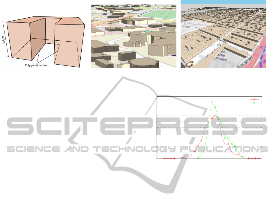
Figure 1: Figure 1(a) illustrate our building model. Figures 1(b) and 1(c) are examples of views generated by our implemen-
tation.
constraint and parametrize it with only 2 angles: az-
imuth and elevation which are defined relative to the
north (respectively horizon) and positive toward east
(respectively zenith).
3.1 Sun Position Computation
Algorithm
Even if it seems easy at first glance, prediction of
the sun position can be affected by many perturba-
tions: influence of the moon causing precession and
nutation, decreasing rotation speed of the earth, at-
mospheric refraction, etc. Authors have proposed
various algorithms (Michalsky, 1988; Blanco-Muriel
et al., 2001; Reda and Andreas, 2008; Grena, 2008)
reflecting different trade-off between accuracy of pre-
diction (within a given period of validity) and com-
plexity of the model. Most recent work comes from
(Grena, 2012) which provides five new algorithms, of
various complexity, targeting the 2010-2110 period.
We base our work on the third proposed algorithm be-
cause it achieves the best trade-off between accuracy
(max error of 0.009
◦
) and complexity.
Besides latitude, longitude, and time of observa-
tion (year, month, day and decimal hour), this algo-
rithm expects temperature, pressure and ∆T = TT −
UT. Pressure and Temperature are used for refraction
correction, whereas ∆T accounts for earth rotation ir-
regularity. In our implementation, we have chosen,
in order to reduce parameters number, to fix them to
reasonable approximations: 25
◦
C, 1 atm and 67s re-
spectively. See http://maia.usno.navy.mil/ for
values of ∆T.
3.2 Results
In order to validate our implementation, we used datas
provided by the Institut de m
´
ecanique c
´
eleste et de
calcul des
´
eph
´
em
´
erides (referred as IMCCE here-
after) as reference. However, we had to remove at-
0
0.02
0.04
0.06
0.08
0.1
0.12
0.14
0.16
0.18
0.2
-0.015 -0.01 -0.005 0 0.005 0.01
frequency [no unit]
error [in deg]
azimuth (µ=-0.0017)
elevation (µ=-0.0005)
Figure 2: Error distribution of azimuth and elevation angles.
mospheric refraction correction from our implemen-
tation, for this comparison, because IMCCE dataset
was built without considering such a correction.
We acquired 10000 values (1 hour spaced) of sun
position during the year 2013-2014 at a specific GPS
coordinate (Lyon, FRANCE) and verified that our im-
plementation matched IMCCE dataset.
The distribution error for the year 2013 shown
in figure 2 confirms the high accuracy of the algo-
rithm: azimuth absolute error stays below 0.009
◦
and
elevation below 0.006
◦
. However both azimuth and
elevation suffer from a negative bias (-0.0017
◦
and -
0.0005
◦
respectively). One of the possible cause of
this bias is that we sample in a very narrow subdomain
of algorithm parameters domain: time parameters are
only taken at the very beginning of the time validity
domain and localization parameters are the same for
all samples.
Given the very low error on azimuth and elevation,
we consider that our implementation is correct. vfill
4 CAMERA MODEL
The purpose of the camera model is to produce a syn-
thetic view of the scene, as seen by the real camera.
VISAPP2013-InternationalConferenceonComputerVisionTheoryandApplications
604
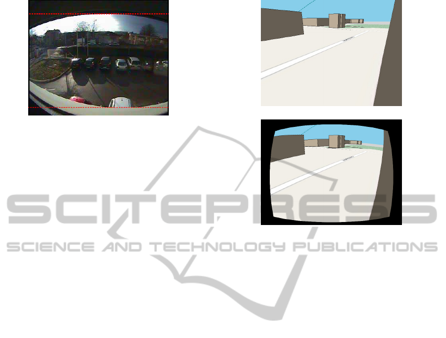
Figure 3: An example of severe lens distortion. Red dotted
lines serve as a straight reference.
Because of its generality and wide use, we have cho-
sen the Hartley-Zisserman (Hartley and Zisserman,
2003) formulation of the pinhole camera model to
generate cameras views of the scene.
Furthermore, we encountered, especially in case
of camera with short focals, prominent non-linear lens
distortion which needed to be modelled as well, as
shown in figure 3.
We employed the Brown-Conrady (Brown, 1966)
distortion model which allows radial and tangential
components of lens distortion to be taken into ac-
count:
x
d
y
d
= (1+k
1
r
2
u
+ k
2
r
4
u
)
x
u
y
u
+
2p
1
x
u
y
u
+ p
2
(r
2
u
+ 2x
2
u
)
2p
2
x
u
y
u
+ p
1
(r
2
u
+ 2y
2
u
)
(2)
In equation 2, (x
u
,y
u
) and (x
d
,y
d
) denotes undis-
torted and distorted coordinates respectively; r
2
u
=
x
2
u
+ y
2
u
is the distance to the principal point (which
is assumed to be the same as the distortion center);
k
1
, k
2
are the radial component parameters and p
1
, p
2
are the tangential component parameters.
An illustration of the rendering with and without
distortion is given in figure 4
5 RESULTS
Purpose of this section is to assess performance of
our shadow prediction model. To this effect, we will
compare qualitatively and quantitatively our synthetic
camera view generated using OpenGL to the corre-
sponding real camera image. We present below two
examples featuring different scene contexts and time
scales.
Our first example (referred as parking hereafter)
shows performances of our model in an urban context
where OpenStreetMap data are available. Therefore,
we extracted data from OpenStreetMap and manu-
ally edited missing building heights with reasonable
values (some buildings were hidden behind a wall
and were therefore given a height of 0m to avoid
(a) Original view
(b) Distorted view
Figure 4: Illustration of lens distortion rendering.
their effect). We set manually camera parameters to
match real camera conditions. The sequence runs
from 18/07/2012 14h to 19/07/2012 11h.
Our second example (referred as dam hereafter),
takes place at an hydroelectric dam and shows perfor-
mances on a wider time scale: we used a sequence
running from 2/5/2011 to 9/27/2011. However, this
time, OpenStreetMap data were not sufficient and had
to be manually edited: We used a satellite view of the
zone as a reference to draw the building outline. We
faced furthermore a subtle problem: in our model,
shadows are projected on the ground which is the
plane z = 0. In this context it means the water is at
z = 0. However, at the dam the water level varies (up
to 3 meters according to our tests) which caused a loss
of performance. To keep our model with projection
plane at z = 0, we adapted the dam and camera height
to reflect water level changes.
5.1 Qualitative Results
Visual comparison shows encouraging results for the
two sequences especially when lens distortion is taken
into account: shadows almost match in shape and ori-
entation.
When lens distortion is omitted, buildings do not
match the real picture and shadows are offseted. This
effect is very noticeable in the first picture of first row
for instance, or in upper-left corner of images from
third row.
APrior-knowledgebasedCastedShadowsPredictionModelFeaturingOpenStreetMapData
605
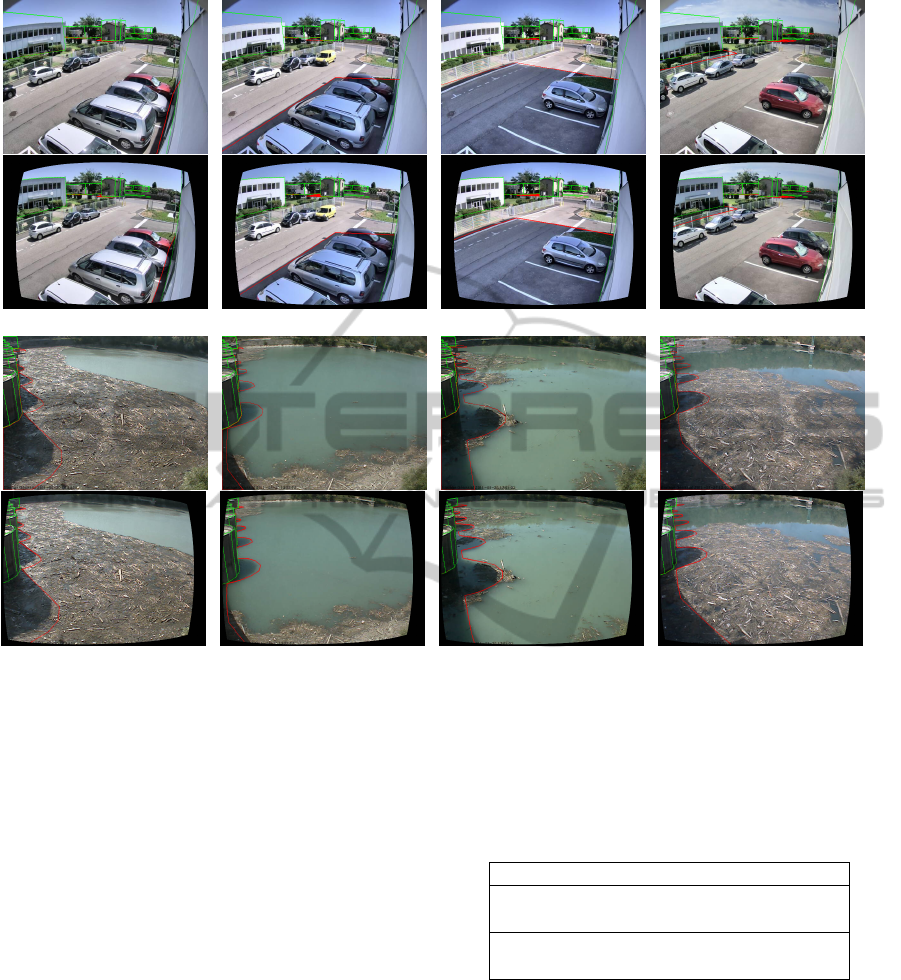
(e) 07/18/2012 13:58:56 (f) 07/18/2012 16:19:56 (g) 07/18/2012 18:21:29 (h) 07/19/2012 10:46:31
(m) 30/06/2011 18:34:08 (n) 30/07/2011 13:52:12 (o) 28/08/2011 17:01:33 (p) 27/09/2011 13:00:35
Figure 5: Visual comparison of predicted buildings (outlined in green) and corresponding shadows (outlined in red). First
(resp. third) row compares prediction and real image when no distortion is applied in the parking (resp. dam) sequence.
Second (resp. fourth) row compares prediction and real image when lens distortion is applied in the parking (resp. dam)
sequence. (Best viewed in color).
5.2 Quantitative Results
In order to conduct our quantitative evaluation, we
manually segmented building shadows casted on the
ground in the camera image using the following rules:
• We discarded the black border region caused by
our lens distortion implementation.
• We considered only shadows of building casted on
the ground.
• When objects such as cars, fences or bushes oc-
cluded the potential ground shadow region, if
there was no ambiguity, we extended known shad-
ows boundaries, otherwise we discarded ambigu-
ous pixels.
Then we compared our prediction and the afore-
mentioned ground-truth on a pixel basis and derived
common metrics such as Coverage Ratio (CR) (also
known as Jaccard index), Precision (P), Recall (R)
Table 1: Quantitative evaluation of performance. Row 1
and 2 (respectively 3 and 4) show results with (respectively
without) lens distortion. All values are expressed in percent.
Sequence CR P R F-score
Parking 85.1 94.4 89.3 91.7
Dam 82.1 88.4 91.8 89.9
Parking 66.5 74.6 77.6 76.0
Dam 78.1 85.6 89.7 87.2
and F-score. We give average results for each context
in table 1.
Quantitative results confirm promising results
shown in the qualitative evaluation and bolster the
contribution of lens distortion.
6 CONCLUSIONS
In this article we presented a prior-knowledge based
building shadow prediction model which features: a
VISAPP2013-InternationalConferenceonComputerVisionTheoryandApplications
606

scene model built with OpenStreetMap datas, a high
precision shadow model and a camera model includ-
ing lens distortion. We showed qualitative and quan-
titative results of this approach. While results are
promising, pixel-precision can’t be achieved easily
with this sole approach, because many parameters
need to be set accurately: building outlines are re-
trieved from OpenStreetMap which makes no guar-
anty of accuracy and camera calibration can be tricky
especially given the high number of degree of free-
dom (3 for camera position, 3 for camera orienta-
tion, 5 for intrinsic parameters and 4 for lens distor-
tion). However, we insist on the fact that this build-
ing shadow prediction model is the first step to a more
general approach which will match predicted shadows
to unknown moving shadows, and therefore pixel-
precision results should not be required.
Furthermore, in this article we only focused on the
shadow prediction part whereas much more informa-
tion is available from our model. Indeed, because of
the geometrical nature of our scene model, we have
access to the depth map and occlusion mask quite eas-
ily. We will investigate, in future work, how can we
make use of such information, especially in an object
tracking context.
REFERENCES
Blanco-Muriel, M., Alarc
´
on-Padilla, D. C., L
´
opez-
Moratalla, T., and Lara-Coira, M. (2001). Computing
the solar vector. Solar Energy, 70(5):431–441.
Blinn, J. (1988). Me and my (fake) shadow. IEEE Comput.
Graph. Appl., 8(1):82–86.
Brown, D. C. (1966). Decentering Distortion of Lenses.
Photometric Engineering, 32(3):444–462.
Cucchiara, R., Grana, C., Piccardi, M., Prati, A., and Sirotti,
S. (2001). Improving shadow suppression in moving
object detection with HSV color information. In In-
telligent Transportation Systems, 2001. Proceedings.
2001 IEEE, pages 334–339.
Finlayson, G. D., Hordley, S. D., Lu, C., and Drew, M. S.
(2002). Removing shadows from images. In In
ECCV 2002: European Conference on Computer Vi-
sion, pages 823–836.
Finlayson, G. D., Hordley, S. D., Lu, C., and Drew, M. S.
(2006). On the removal of shadows from images.
IEEE Transactions on Pattern Analysis and Machine
Intelligence, 28:59–68.
Grena, R. (2008). An algorithm for the computation of the
solar position. Solar Energy, 82(5):462–470.
Grena, R. (2012). Five new algorithms for the computa-
tion of sun position from 2010 to 2110. Solar Energy,
86(5):1323–1337.
Hartley, R. and Zisserman, A. (2003). Multiple View Geom-
etry in Computer Vision. Cambridge University Press,
New York, NY, USA, 2 edition.
Huang, J.-B. and Chen, C.-S. (2009). Moving cast shadow
detection using physics-based features. Computer Vi-
sion and Pattern Recognition, IEEE Computer Society
Conference on, 0:2310–2317.
Jackson, B., Bodor, R., and Papanikolopoulos, N. (2004).
Learning static occlusions from interactions with
moving figures. In Intelligent Robots and Systems,
2004. (IROS 2004). Proceedings. 2004 IEEE/RSJ In-
ternational Conference on, volume 1, pages 963–968
vol.1. IEEE.
Kaneva, B., Torralba, A., and Freeman, W. T. (2011). Eval-
uating image feaures using a photorealistic virtual
world. In IEEE International Conference on Com-
puter Vision.
Lalonde, J.-F., Efros, A. A., and Narasimhan, S. G. (2009).
Estimating natural illumination from a single outdoor
image. In IEEE International Conference on Com-
puter Vision.
Leone, A. and Distante, C. (2007). Shadow detection for
moving objects based on texture analysis. Pattern
Recogn., 40:1222–1233.
Leotta, M. J. and Mundy, J. L. (2006). Learning background
and shadow appearance with 3-D vehicle models. In
Proc. British Machine Vision Conference (BMVC).
Marin, J., Vazquez, D., Geronimo, D., and Lopez, A. M.
(2010). Learning appearance in virtual scenarios for
pedestrian detection. Computer Vision and Pattern
Recognition, IEEE Computer Society Conference on,
0:137–144.
Michalsky, J. J. (1988). The astronomical almanac’s algo-
rithm for approximate solar position (19502050). So-
lar Energy, 40(3):227–235.
Nadimi, S. and Bhanu, B. (2004). Physical models for mov-
ing shadow and object detection in video. IEEE trans-
actions on Pattern Analysis and Machine Intelligence
(PAMI), 26(8).
OpenStreetMap contributors (2012a). http://taginfo.
openstreetmap.org/keys/building.
OpenStreetMap contributors (2012b). http://
www.openstreetmap.org.
Reda, I. and Andreas, A. (2008). Solar position algorithm
for solar radiation applications.
Sanin, A., Sanderson, C., and Lovell, B. (2012). Shadow
detection: A survey and comparative evaluation of re-
cent methods. Pattern Recognition, 45:1684–1695.
APrior-knowledgebasedCastedShadowsPredictionModelFeaturingOpenStreetMapData
607
