Image Guided Cost Aggregation for Hierarchical Depth Map Fusion

Thilo Borgmann and Thomas Sikora

Communication Systems Group, Technische Universit

at Berlin, Berlin, Germany

Keywords:

Multi View Stereo, Stereo Matching, Depth Estimation, Depth Map Fusion.

Abstract:

Estimating depth from a video sequence is still a challenging task in computer vision with numerous applica-

tions. Like other authors we utilize two major concepts developed in this ﬁeld to achieve that task which are

the hierarchical estimation of depth within an image pyramid as well as the fusion of depth maps from different

views. We compare the application of various local matching methods within such a combined approach and

can show the relative performance of local image guided methods in contrast to commonly used ﬁxed–window

aggregation. Since efﬁcient implementations of these image guided methods exist and the available hardware

is rapidly enhanced, the disadvantage of their more complex but also parallel computation vanishes and they

will become feasible for more applications.

1 INTRODUCTION

Reconstructing a three–dimensional representation of

a scene from multiple images of a video sequence

is one of the most important topics in computer vi-

sion. It serves as an essential basis for numerous ap-

plication from different areas like robotics, medical

imaging, video processing and many more. Intense

research on this topic has been done for many years

and the state–of–the–art advances rapidly. Yet it is

still a challenging task to acquire high–quality 3D re-

constructions using image–based methods only.

The enormous amount of algorithms proposed to

accomplish this task use a wide variety of approaches.

The most important property to distinguish between

these algorithms is their scope of matching and opti-

mization, either locally or globally. This categoriza-

tion holds in general, even though there are some ap-

proaches in between. Algorithms utilizing a global

optimization tend to produce the most accurate re-

sults. Unfortunately, achieving this quality usually re-

quires complex computations and is therefore not al-

ways feasible with respect to the desired application.

Also, these algorithms usually provide limited capa-

bilities of parallelization. Thus even modern com-

puter hardware cannot compensate this drawback due

to their still limited computation of sequential parts of

these algorithms.

In contrast to these methods, algorithms based on

local matching approaches are much less complex and

offer the advantage of rapid computation. Although

they usually suffer from the ambiguities within their

local scope. Early approaches show a severe differ-

ence in quality compared to their globally optimized

counterparts. However, recent improvements to local

matching can signiﬁcantly reduce the gap between the

two categories. Always considering a limited local

area only, these methods also offer excellent possibil-

ities for parallelization. Modern computer hardware

in turn provide a basis for such massive parallel com-

putation so that the number of high–quality real–time

capable algorithms permanently increase.

For a comprehensive overview of existing meth-

ods and their relative performance evaluation, we re-

fer to the publicly available benchmarks covering this

topic (Scharstein et al., 2001) (Seitz et al., 2006)

(Strecha et al., 2008).

Nevertheless, there is always the trade–off be-

tween quality and computational complexity. Given

a set of calibrated images from a video sequence,

we utilize two major concepts developed in this area,

which are the hierarchical estimation of depth maps

(Yang and Pollefeys, 2003) (Zach et al., 2004) (Cor-

nelis and Van Gool, 2005) (Nalpantidis et al., 2009)

and the fusion of depth maps from multiple views

(Zitnick et al., 2004) (Merrell et al., 2007) (Zach,

2008) (Zhang et al., 2009) (Unger et al., 2010).

The fusion of the depth maps allows to achieve

a high quality while the hierarchical structure of the

depth estimation helps to reduce complexity. We are

not the ﬁrst to combine these approaches (McKinnon

et al., 2012). The authors evaluated the inﬂuence of

199

Borgmann T. and Sikora T..

Image Guided Cost Aggregation for Hierarchical Depth Map Fusion.

DOI: 10.5220/0004212901990207

In Proceedings of the International Conference on Computer Vision Theory and Applications (VISAPP-2013), pages 199-207

ISBN: 978-989-8565-48-8

 2013 SCITEPRESS (Science and Technology Publications, Lda.)

several parameters to their approach but the choice

of the initial depth map estimation and cost aggre-

gation is just roughly covered. The several authors

of the former contributions about hierarchical estima-

tion and depth map fusion do also not report compara-

tively about different estimation approaches. Thus, in

contrast to other methods, our contribution is to reveal

the relative performance of the applied cost aggrega-

tion used throughout the hierarchical estimation pro-

cess instead of focusing on a sophisticated process-

ing on or between the higher levels of the approach.

Although a global matching algorithm seems feasible

at that stage of the hierarchical processing, the rel-

ative overhead remains and we stick to local meth-

ods. We therefore implemented and compared the

performance of several well–known cost aggregation

methods that have already been proven their ability to

achieve high-quality estimation results as well as be-

ing computational efﬁcient. We integrate them into a

rather simple hierarchical scheme for the applied cost

aggregation to be the dominant factor within this pro-

cess. This leads us to the relative performance of the

initial depth map and cost aggregation used in such a

hierarchical framework.

2 RELATED WORK

Common two–view disparity estimation algorithms

compute separate disparity maps for each of the

two views, postprocessed by a left–right consistency

check. By applying that, ambiguous matches and oc-

cluded pixels are detected. This approach has also

been transfered and adapted for depth estimation in

multi–view matching (Zitnick et al., 2004) (Merrell

et al., 2007).

Hierarchical disparity matching is also a common

approach in the ﬁeld of stereo matching. In (Yang

and Pollefeys, 2003) (Zach et al., 2004) (Cornelis and

Van Gool, 2005) the authors successfully demonstrate

the real–time capabilities and efﬁciency of their ap-

proaches.

A combination of the former methods is pre-

sented in (McKinnon et al., 2012). The authors

describe an iterative approach of the fusion of

depth maps throughout their hierarchical estimation

scheme. Within each level of the hierarchy, the depth

map is further reﬁned by an iterative application of

the connectivity constraint (Cornelis and Van Gool,

2005).

Many cost aggregation methods have been pro-

posed based on variable support regions (Tombari

et al., 2008a). Among many that dynamically select

different or multiple support windows (Hirschm

uller

et al., 2002) or varying window sizes (Veksler, 2003),

we concentrate on those approaches that deﬁne the

support region based on the local surrounding within

the image like (Yoon and Kweon, 2006) (Tombari

et al., 2008b) (Zhang et al., 2009) (He et al., 2010).

We refer to these as image guided aggregation meth-

ods.

Cost aggregation methods are amongst the most

important things to consider for stereo matching algo-

rithms. According to the rapid development of these

algorithms, cost aggregation methods are also rapidly

enhanced. Next to benchmarks like (Scharstein et al.,

2001) (Strecha et al., 2008), which evaluate complete

algorithms, the bare cost initialization and aggrega-

tion methods have also been addressed by other con-

tributions.

In (Wang et al., 2006) the authors evaluate a set

of well–known cost initialization methods in combi-

nation with image guided and unguided cost aggrega-

tions. They use several sequences from the Middle-

burry stereo data set to compare the resulting dispar-

ity estimations. All methods are evaluated by being

incorporated into the same disparity estimator. Con-

cerning the evaluated image guided cost aggregation

methods they approve the expected gain in quality of

the disparity estimation. They also show the increas-

ing complexity when using these methods.

A very comprehensive evaluation of cost initial-

izations and cost aggregations as well as their rela-

tion to each other has been done in (Tombari et al.,

2008a). Many different image guided aggregation

methods have been evaluated also using the Middle-

burry stereo data set. They use a simplistic winner–

takes–all approach to generate their results for a clear

dependency on the incorporated initialization and ag-

gregation methods. We instead do not only cover the

quality of the generated depth map but also the in-

ﬂuence of repeatedly applied depth map fusion and

reﬁnement using the corresponding cost and aggrega-

tion methods.

3 HIERARCHICAL ALGORITHM

For our hierarchical implementation, we adopt several

techniques from previous approaches of (Cornelis and

Van Gool, 2005) and (McKinnon et al., 2012).

We iterate through an image pyramid. Each level

k of the pyramid holds frames of half the width and

height of the size of the succeeding level. In this im-

plementation, we reduce the resolution for the lowest

level of the pyramid to 1 / 64th of the full resolution.

Due to our hardware limitations, we have to restrict

the highest level of the pyramid to 1 / 4th of the full

VISAPP2013-InternationalConferenceonComputerVisionTheoryandApplications

200

resolution (1536x1024 pixels).

For the ﬁrst level k = 0 of this hierarchy, we ap-

ply an initial plane–sweep based estimation. For each

succeeding level k > 0, we apply a reﬁning depth map

based sweep adopted from (Cornelis and Van Gool,

2005). The depth estimates of the current level are

then processed by a depth map fusion before the algo-

rithm proceeds to the next level in the hierarchy. For

that, all depth estimates of the current level have to

be concurrently computed. After the ﬁrst level k = 0

has been processed, the parameters r

and d

that in-

ﬂuence the reﬁning depth map sweep used in all lev-

els k > 0 are updated according to the current level.

This hierarchical approach can be seen as a simpli-

ﬁed variant of the scheme presented in (McKinnon

et al., 2012) with just one reﬁnement iteration within

the levels of the hierarchy.

The following pseudo code outlines the described

algorithm:

For all lev els k

For all ca m er as

If k = 0 then

Ini ti a l Dep t h E s ti ma ti on

Else

= k * r

= 1/2 * d

k−1

Dept h Map Swe ep

Dept h Map Fu sio n

End

In the following sections we brieﬂy outline each

individual step and describe the inﬂuence of the pa-

rameters r

and d

3.1 Initial Depth Estimation

For each camera, we basically apply a fronto–parallel

plane–sweep approach (Collins, 1996). We divide

the sequence into two halves for the preceding and

succeeding views according to (Kang et al., 2001).

The number of views projected onto the sweep–

plane might vary, but we found using one view to

be sufﬁcient. The sweep–plane is then projected into

the reference camera and for each depth the photo–

consistency function according to the applied cost and

aggregation methods is computed.

Throughout all depths we apply a simple winner–

takes–all approach to receive the minimal cost for

each pixel. A simple parabolic interpolation is applied

using the depth and cost values of the sweep–layers in

front and behind the minimum plane to achieve a con-

tinuous depth value.

A second sweep follows with the projecting view

used as the reference view to apply a standard

left–right consistency check to remove ambiguous

matches. This bidirectional sweeping procedure is ap-

plied using the preceding as well as the succeeding

views. The combination of both intermediate depth

maps D

i,L

, D

i,R

results in a continuous depth map

for each reference view D

= D

i,L

i,R

. Note that

one of these bidirectional sweeps can be reused for

the depth map estimation of the succeeding reference

view: D

i−1,R

= D

i,L

. Thus, for each camera pair of the

sequence just one bidirectional sweep has to be com-

puted. The initial depth estimation is followed by the

ﬁrst depth map fusion that is equal to all levels.

3.2 Depth Map Sweep

The fused depth maps from the previous level k − 1

are swept again using the current resolution within a

small range d

around the current depth estimate (Cor-

nelis and Van Gool, 2005). This range around the esti-

mate is decreased to half the size of the previous level:

k−1

(1)

The respective window or kernel sizes s depend on

a given parameter r

, so that s = (2r

+ 1)

. For the

cross–based method of (Zhang et al., 2009), r

deﬁnes

the maximum arm length used. The value of r

linearly increased by the current level on basis of the

initial size:

= kr

(2)

For the image guided aggregation methods, a sec-

ond parameter e is required that controls the image

guided creation of the support region. This parame-

ter is ﬁxed for all applications of the corresponding

aggregation but differs according to the method used.

However, for our simpliﬁed hierarchical approach we

rely on the reﬁned sampling interval and the enforced

smoothness during the fusion stage to enhance the es-

timation and do not incorporate a connectivity con-

straint.

3.3 Depth Map Fusion

In this stage the depth maps of the surrounding views

generated in the same level are projected into the ref-

erence view. We apply only two simple validations to

reject outliers from being candidates for the fusion.

First, we accept only candidates that are within a

close distance ε to the reference estimation and there-

fore support its location (Merrell et al., 2007). Sec-

ond, the euclidean distance between the color vectors

of the reference pixel and the candidate pixel is tested

to be within another threshold θ. From the set of re-

maining candidates, we apply another winner–takes–

ImageGuidedCostAggregationforHierarchicalDepthMapFusion

201

0%#

5%#

10%#

15%#

20%#

25%#

30%#

35%#

40%#

45%#

50%#

ADC#

OPT#

ADC#

OPT#

SAD#

SSD#

NCC#

CB#

GF#

Level#0#

Final#

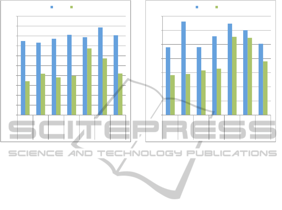
Figure 1: Comparison of the fusion results of all combina-

tions using their respective best performing parameters for

‘Fountain’.

all approach to select the candidate with the smallest

cost value corresponding to its origin view.

The last step is to apply a mean ﬁlter to smooth

the fused depth maps. To preserve depth discontinu-

ities, we compute this ﬁlter within a cross–based sup-

port region generated by (Zhang et al., 2009) using

a small maximum arm length r

. The used parame-

ters θ, ε and r

are constant for all levels. The fused

depth maps are then passed to the next iteration on the

succeeding level.

4 EVALUATION

We compare several approaches for cost initializa-

tion and cost aggregation used to compute the photo–

consistency function during the plane-sweeps.

Some of the most common combinations are the

absolute intensity differences and the squared inten-

sity differences, aggregated within a ﬁxed–window

to form the well–known sum of absolute differences

(SAD) and sum of squared differences (SSD) cost

functions. Next to these, there is also the normalized

cross–correlation (NCC) to be considered in this cat-

egory.

For the comparison with image guided cost func-

tions, we have chosen two state–of–the–art ap-

proaches. The ﬁrst is the guided image ﬁltering (GF)

approach presented in (He et al., 2010). The second is

the cross–based aggregation method (CB) of (Zhang

0%#

10%#

20%#

30%#

40%#

50%#

60%#

70%#

ADC#

OPT#

ADC#

OPT#

SAD#

SSD#

NCC#

CB#

GF#

Level#0#

Final#

Figure 2: Comparison of the fusion results of all combina-

tions using their respective best performing parameters for

‘Herz–Jesu’.

et al., 2009). Among many alternatives to these ag-

gregation methods, these two have proven to perform

very accurately in state–of–the–art stereo matching

algorithms (Rhemann et al., 2011) (Mei et al., 2011)

and also provide very efﬁcient implementations using

integral images (Crow, 1984). In (Mei et al., 2011) the

cross–based aggregation is applied to a cost initializa-

tion based on a linear combination of the absolute dif-

ferences and the census transform called AD–Census

(ADC). In (Rhemann et al., 2011) a common cost ini-

tialization based on the absolute differences and gra-

dients (OPT) is used, well–known from many contri-

butions concerning the optical ﬂow computation.

Therefore we include in our comparison both

these combinations (CB + ADC, GF + OPT) as well

as the combination of exchanged initialization and ag-

gregation methods (CB + OPT, GF + ADC). Thus, we

have a set of seven combinations to be evaluated in

our hierarchical framework.

We have chosen two well–known wide–baseline

outdoor sequences from the data set provided by

(Strecha et al., 2008) for our evaluation: ‘Fountain’

and ‘Herz-Jesu’. These sequences feature a ground–

truth 3D–model, acquired using a laser range scanner,

and ground-truth camera calibration. We measure the

quality of our results by projecting the ground–truth

model into all processed cameras of the sequence. For

each pixel the resulting depth value of that projection

is then compared to the depth values generated by our

hierarchical algorithm. We generate a histogram of

VISAPP2013-InternationalConferenceonComputerVisionTheoryandApplications

202

0%#

10%#

20%#

30%#

40%#

50%#

60%#

70%#

80%#

90%#

100%#

10#

11#

CB#+#ADC#

CB#+#OPT#

GF#+#ADC#

GF#+#OPT#

NCC#

SSD#

SAD#

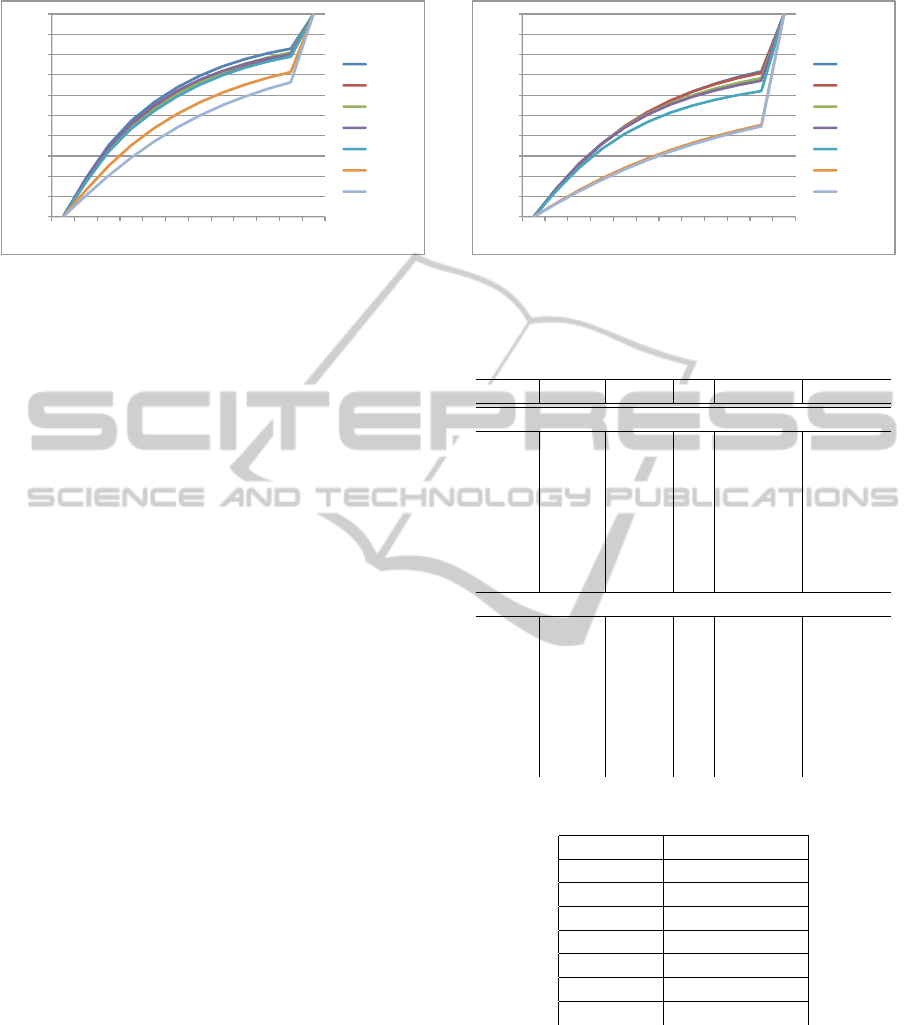
Figure 3: Cumulative distribution of best performing com-

binations for sequence ‘Fountain’.

eleven bins to accumulate pixels according to their

depth difference. Like (McKinnon et al., 2012), we

deﬁne a threshold σ equivalent to 3mm for each bin of

the histogram. All estimates with a difference greater

than 10σ as well as all missing pixels according to

the ground–truth are accumulated in the last bin. This

histogram is closely related to the evaluation scheme

used in (Strecha et al., 2008) and (McKinnon et al.,

2012). It reveals the precision of the estimated pix-

els as well as the completeness in terms of the given

threshold of 10σ.

We compare the various combinations of cost and

aggregation methods primarily by their amount of

precisely estimated pixels. For that we can utilize

the last bin of the histogram. The lower that value

the more pixels have been estimated with a sufﬁcient

precision and the better the aggregation method per-

forms. The values presented are given by percentage

of all pixels estimated. In ﬁgure 1 and ﬁgure 2 we

compare the best performing parameters for all seven

combinations applied to the according sequence. For

each combination, the result after the ﬁrst depth map

fusion at level k = 0 and the result of the ﬁnal depth

map fusion are shown. This illustrates the overall per-

formance as well as the beneﬁts of the hierarchical

processing. The corresponding parameters are given

in table 1. In ﬁgure 3 and ﬁgure 4 we show the ac-

cording cumulative distribution to visualize the rel-

ative precision for these combinations, too. For the

best and worst performing image guided and ﬁxed

methods, we show the color–coded differences to the

ground-truth for a subimage of both sequences in ﬁg-

ure 5. The pixel–wise differences are color–coded ac-

cording to bins of the corresponding histogram, from

white for small differences less or equal to σ to black

for differences up to 10σ. All blue pixels represent

differences of more than 10σ.

We use the parameters given in table 2 for the

complete evaluation. The parameters r

and e in-

ﬂuence the behavior of the aggregation methods and

0%#

10%#

20%#

30%#

40%#

50%#

60%#

70%#

80%#

90%#

100%#

10#

11#

CB#+#ADC#

CB#+#OPT#

GF#+#ADC#

GF#+#OPT#

NCC#

SSD#

SAD#

Figure 4: Cumulative distribution of best performing com-

binations for sequence ‘Herz–Jesu’.

Table 1: Best performing parameter values for each combi-

nation and sequence.

Agg. Cost e r

Level 0 Final

Fountain:

CB ADC 12 3 37,4383 17,1133

CB OPT 12 3 36,6367 20,8848

GF ADC 0,001 1 38,6234 19,0225

GF OPT 0,001 2 40,5867 19,8058

SAD 1 39,3672 33,6869

SSD 2 44,3056 28,6606

NCC 2 40,3505 21,0151

Herz–Jesu:

CB ADC 5 1 48,0009 28,2878

CB OPT 5 2 66,2230 29,0251

GF ADC 0,100 1 48,0823 31,6208

GF OPT 0,100 1 55,7852 32,8818

SAD 1 64,7667 55,4109

SSD 2 60,1193 54,7170

NCC 1 50,4895 37,9934

Table 2: Parameter values used for the parameter-sweep.

Parameter Value(s)

θ 0.2

0.3

ε 0.1

1, 2, 3, 4, 6

e(GF) 0.1,0.01, 0.001

e(CB) 5, 8, 12

are therefore assigned several values for a parameter–

sweep. Note that e depends on the image guided

method and has completely different values assigned.

For the guided image ﬁlter (He et al., 2010), this value

is similar to ε of the original implementation. For

the cross–based aggregation (Zhang et al., 2009), this

value corresponds to τ.

ImageGuidedCostAggregationforHierarchicalDepthMapFusion

203

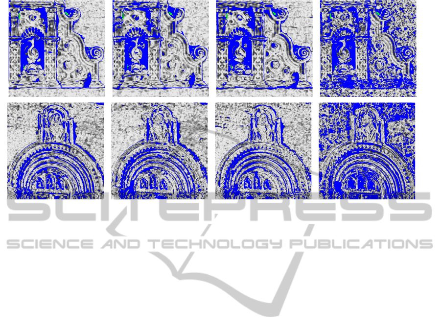
(a) CB + ADC (b) GF + OPT (c) NCC (d) SAD

Figure 5: Subimages of both sequences showing the pixel–wise evaluation by color–coded differences to the ground–truth.

Differences range from ≤ 1σ (white) to ≤ 10σ (black). Blue color indicates a difference of > 10σ. Sequence ‘Fountain’

is shown in the upper row, sequence ‘Herz–Jesu’ is shown in the lower row. The best (a) and the worst (b) image guided

combinations as well as the best (c) and the worst (d) ﬁxed methods are shown.

5 CONCLUSIONS

We can show in our evaluation that the applica-

tion of image guided methods generally produce a

more complete and precise result, see ﬁgures 1, 2,

3, 4 and 5. For the ‘Fountain’ sequence, the differ-

ence between the best performing image guided and

non–guided method is around 4%, and almost 10%

for ‘Herz–Jesu’. Although the normalized cross–

correlation performs almost as well as the image

guided approach (GF + OPT) on the ‘Fountain’ se-

quence, the difference becomes larger in a more

complex sequence like ‘Herz–Jesu’. Nevertheless, it

clearly outperforms the SAD and SSD approaches on

both sequences.

Thus, the application of image guided methods

has its beneﬁts although they require a slightly more

complex computation. However, this disadvantage

vanishes due to the improving hardware capabili-

ties in terms of parallel computing. The normalized

cross–correlation offers a good trade–off between

quality and complexity for both sequences. These re-

sults encourage us to further investigate the applica-

tion of image guided methods in a more sophisticated

hierarchical estimation approach.

ACKNOWLEDGEMENTS

The authors like to thank David M

Kinnon, Ryan

Smith and Ben Upcroft for their most valuable sup-

port of various data and personal contact.

REFERENCES

Collins, R. (1996). A space-sweep approach to true

multi-image matching. In Computer Vision and Pat-

tern Recognition, 1996. Proceedings CVPR’96, 1996

IEEE Computer Society Conference on, pages 358–

363. IEEE.

Cornelis, N. and Van Gool, L. (2005). Real-time connec-

tivity constrained depth map computation using pro-

grammable graphics hardware. In Computer Vision

and Pattern Recognition, 2005. CVPR 2005. IEEE

Computer Society Conference on, volume 1, pages

1099–1104. IEEE.

Crow, F. (1984). Summed-area tables for texture mapping.

ACM SIGGRAPH Computer Graphics, 18(3):207–

212.

He, K., Sun, J., and Tang, X. (2010). Guided image ﬁltering.

Computer Vision–ECCV 2010, pages 1–14.

Hirschm

uller, H., Innocent, P., and Garibaldi, J. (2002).

Real-time correlation-based stereo vision with re-

duced border errors. International Journal of Com-

puter Vision, 47(1):229–246.

Kang, S., Szeliski, R., and Chai, J. (2001). Handling occlu-

sions in dense multi-view stereo. In Computer Vision

VISAPP2013-InternationalConferenceonComputerVisionTheoryandApplications

204

and Pattern Recognition, 2001. CVPR 2001. Proceed-

ings of the 2001 IEEE Computer Society Conference

on, volume 1, pages I–103. IEEE.

McKinnon, D., Smith, R., and Upcroft, B. (2012). A semi-

local method for iterative depth-map reﬁnement. In

Proceedings of the IEEE International Conference on

Robotics and Automation (ICRA 2012). IEEE.

Mei, X., Sun, X., Zhou, M., Jiao, S., Wang, H., and Zhang,

X. (2011). On building an accurate stereo matching

system on graphics hardware. In Computer Vision

Workshops (ICCV Workshops), 2011 IEEE Interna-

tional Conference on, pages 467–474. IEEE.

Merrell, P., Akbarzadeh, A., Wang, L., Mordohai, P.,

Frahm, J., Yang, R., Nist

er, D., and Pollefeys, M.

(2007). Real-time visibility-based fusion of depth

maps. In Computer Vision, 2007. ICCV 2007. IEEE

11th International Conference on, pages 1–8. Ieee.

Nalpantidis, L., Amanatiadis, A., Sirakoulis, G., Kyriak-

oulis, N., and Gasteratos, A. (2009). Dense dispar-

ity estimation using a hierarchical matching technique

from uncalibrated stereo vision. In Imaging Systems

and Techniques, 2009. IST ’09. IEEE International

Workshop on, pages 427 –431.

Rhemann, C., Hosni, A., Bleyer, M., Rother, C., and

Gelautz, M. (2011). Fast cost-volume ﬁltering for vi-

sual correspondence and beyond. In Computer Vision

and Pattern Recognition (CVPR), 2011 IEEE Confer-

ence on, pages 3017–3024. IEEE.

Scharstein, D., Szeliski, R., and Zabih, R. (2001). A tax-

onomy and evaluation of dense two-frame stereo cor-

respondence algorithms. In Stereo and Multi-Baseline

Vision, 2001. (SMBV 2001). Proceedings. IEEE Work-

shop on, pages 131 –140.

Seitz, S., Curless, B., Diebel, J., Scharstein, D., and

Szeliski, R. (2006). A comparison and evaluation

of multi-view stereo reconstruction algorithms. In

Computer Vision and Pattern Recognition, 2006 IEEE

Computer Society Conference on, volume 1, pages

519 – 528.

Strecha, C., von Hansen, W., Van Gool, L., Fua, P., and

Thoennessen, U. (2008). On benchmarking camera

calibration and multi-view stereo for high resolution

imagery. In Computer Vision and Pattern Recognition,

2008. CVPR 2008. IEEE Conference on, pages 1 –8.

Tombari, F., Mattoccia, S., Di Stefano, L., and Addimanda,

E. (2008a). Classiﬁcation and evaluation of cost ag-

gregation methods for stereo correspondence. In Com-

puter Vision and Pattern Recognition, 2008. CVPR

2008. IEEE Conference on, pages 1–8. IEEE.

Tombari, F., Mattoccia, S., Di Stefano, L., and Addimanda,

E. (2008b). Near real-time stereo based on effective

cost aggregation. In Pattern Recognition, 2008. ICPR

2008. 19th International Conference on, pages 1–4.

IEEE.

Unger, C., Wahl, E., Sturm, P., Ilic, S., et al. (2010). Prob-

abilistic disparity fusion for real-time motion-stereo.

Citeseer.

Veksler, O. (2003). Fast variable window for stereo corre-

spondence using integral images. In Computer Vision

and Pattern Recognition, 2003. Proceedings. 2003

IEEE Computer Society Conference on, volume 1,

pages I–556. IEEE.

Wang, L., Gong, M., Gong, M., and Yang, R. (2006). How

far can we go with local optimization in real-time

stereo matching. In 3D Data Processing, Visualiza-

tion, and Transmission, Third International Sympo-

sium on, pages 129–136. IEEE.

Yang, R. and Pollefeys, M. (2003). Multi-resolution real-

time stereo on commodity graphics hardware. In

Computer Vision and Pattern Recognition, 2003. Pro-

ceedings. 2003 IEEE Computer Society Conference

on, volume 1, pages I–211. IEEE.

Yoon, K. and Kweon, I. (2006). Adaptive support-weight

approach for correspondence search. Pattern Analy-

sis and Machine Intelligence, IEEE Transactions on,

28(4):650–656.

Zach, C. (2008). Fast and high quality fusion of depth

maps. In Proceedings of the International Symposium

on 3D Data Processing, Visualization and Transmis-

sion (3DPVT), volume 1.

Zach, C., Karner, K., and Bischof, H. (2004). Hierarchi-

cal disparity estimation with programmable 3d hard-

ware. In Proc. of WSCG, Pilsen, Czech Republic,

pages 275–282.

Zhang, G., Jia, J., Wong, T., and Bao, H. (2009). Consis-

tent depth maps recovery from a video sequence. Pat-

tern Analysis and Machine Intelligence, IEEE Trans-

actions on, 31(6):974–988.

Zitnick, C., Kang, S., Uyttendaele, M., Winder, S., and

Szeliski, R. (2004). High-quality video view interpo-

lation using a layered representation. In ACM Trans-

actions on Graphics (TOG), volume 23, pages 600–

608. ACM.

APPENDIX

The complete evaluation data is given in separate ta-

bles. There are two tables for each sequence, one for

ﬁxed–window and one for image guided aggregation,

respectively. Tables 3 and 5 show the results for the

sequence ‘Fountain’ and tables 4 and 6 show the re-

sults for the sequence ‘Herz–Jesu’. The values given

in the columns ‘Level 0’ and ‘Final’ are the percent-

ages of pixels estimated with an insufﬁcient precision

after the ﬁrst and ﬁnal depth map fusion, respectively.

ImageGuidedCostAggregationforHierarchicalDepthMapFusion

205

Table 3: Parameter–sweep of image guided aggregation for

the ‘Fountain’ sequence.

Agg. Cost e r

Level 0 Final

CB ADC 5 1 37,7922 21,3303

CB ADC 5 2 39,6136 20,5099

CB ADC 5 3 38,6625 19,3956

CB ADC 5 4 39,418 19,5801

CB ADC 5 6 39,617 17,6259

CB ADC 8 1 37,6795 21,4545

CB ADC 8 2 39,5631 19,9244

CB ADC 8 3 38,295 18,7349

CB ADC 8 4 39,2334 17,7528

CB ADC 8 6 40,1979 18,2764

CB ADC 12 1 37,4367 18,4192

CB ADC 12 2 39,2775 17,5535

CB ADC 12 3 37,4383 17,1133

CB ADC 12 4 39,6574 18,3329

CB ADC 12 6 41,2455 19,3537

CB OPT 5 1 40,0748 25,8658

CB OPT 5 2 38,81 22,9363

CB OPT 5 3 37,6746 21,7772

CB OPT 5 4 38,2792 22,32

CB OPT 5 6 38,0735 20,92

CB OPT 8 1 40,7023 25,9492

CB OPT 8 2 38,2409 21,7358

CB OPT 8 3 37,1505 21,1068

CB OPT 8 4 37,797 21,4484

CB OPT 8 6 39,1751 20,9398

CB OPT 12 1 41,4982 25,3186

CB OPT 12 2 37,9567 21,3778

CB OPT 12 3 36,6367 20,8848

CB OPT 12 4 38,15 21,4235

CB OPT 12 6 40,157 21,5007

GF ADC 0,100 1 40,3396 19,2574

GF ADC 0,100 2 41,895 21,2373

GF ADC 0,100 3 43,4714 24,6391

GF ADC 0,100 4 45,3187 27,7024

GF ADC 0,100 6 49,313 34,1429

GF ADC 0,010 1 39,8775 19,0698

GF ADC 0,010 2 41,4333 20,5663

GF ADC 0,010 3 42,659 23,2175

GF ADC 0,010 4 44,3367 25,9867

GF ADC 0,010 6 48,1713 31,8384

GF ADC 0,001 1 38,6234 19,0225

GF ADC 0,001 2 40,3896 19,2996

GF ADC 0,001 3 41,9276 21,7289

GF ADC 0,001 4 43,5808 24,1429

GF ADC 0,001 6 46,6741 28,7754

GF OPT 0,100 1 38,567 19,9531

GF OPT 0,100 2 43,6802 20,5242

GF OPT 0,100 3 45,5161 32,7966

GF OPT 0,100 4 47,1033 26,9157

GF OPT 0,100 6 50,8852 33,962

GF OPT 0,010 1 38,2503 20,3005

GF OPT 0,010 2 43,0723 20,2045

GF OPT 0,010 3 44,9116 22,2674

GF OPT 0,010 4 46,2428 25,172

GF OPT 0,010 6 49,1156 31,8687

GF OPT 0,001 1 38,4306 21,452

GF OPT 0,001 2 40,5867 19,8058

GF OPT 0,001 3 43,3264 20,8162

GF OPT 0,001 4 44,8305 23,0555

GF OPT 0,001 6 47,3774 28,2155

Table 4: Parameter–sweep of image guided aggregation for

the ‘Herz–Jesu’ sequence.

Agg. Cost e r

Level 0 Final

CB ADC 5 1 48,0009 28,2878

CB ADC 5 2 47,3767 28,2884

CB ADC 5 3 46,8367 28,5651

CB ADC 5 4 47,3276 28,7136

CB ADC 5 6 47,5468 28,5672

CB ADC 8 1 48,1184 29,9848

CB ADC 8 2 47,3707 29,2522

CB ADC 8 3 46,6911 29,4477

CB ADC 8 4 47,5492 29,4454

CB ADC 8 6 48,1225 29,5938

CB ADC 12 1 48,4898 30,3152

CB ADC 12 2 47,2583 29,5847

CB ADC 12 3 46,8833 29,7205

CB ADC 12 4 47,9632 30,0588

CB ADC 12 6 48,9818 30,7885

CB OPT 5 1 71,747 29,2853

CB OPT 5 2 66,223 29,0251

CB OPT 5 3 64,3264 29,3956

CB OPT 5 4 65,0884 29,6815

CB OPT 5 6 60,622 29,4952

CB OPT 8 1 73,0595 35,323

CB OPT 8 2 64,381 34,3963

CB OPT 8 3 62,5112 34,4801

CB OPT 8 4 62,9131 34,3226

CB OPT 8 6 58,353 29,7987

CB OPT 12 1 74,7221 35,5511

CB OPT 12 2 62,9915 34,6381

CB OPT 12 3 59,9426 34,7855

CB OPT 12 4 61,5115 34,746

CB OPT 12 6 57,2033 30,474

GF ADC 0,100 1 48,0823 31,6208

GF ADC 0,100 2 51,1138 33,5118

GF ADC 0,100 3 54,2877 36,0289

GF ADC 0,100 4 57,3762 38,4606

GF ADC 0,100 6 62,8878 40,9152

GF ADC 0,010 1 48,2435 32,5278

GF ADC 0,010 2 50,6403 33,9099

GF ADC 0,010 3 53,485 36,1495

GF ADC 0,010 4 56,2268 38,1879

GF ADC 0,010 6 61,3152 40,5947

GF ADC 0,001 1 48,3742 33,0063

GF ADC 0,001 2 49,9871 33,9849

GF ADC 0,001 3 52,6447 36,0113

GF ADC 0,001 4 55,4582 37,9339

GF ADC 0,001 6 60,3802 40,1883

GF OPT 0,100 1 55,7852 32,8818

GF OPT 0,100 2 53,0231 34,265

GF OPT 0,100 3 55,9169 36,6067

GF OPT 0,100 4 59,4258 38,9416

GF OPT 0,100 6 64,8294 41,5739

GF OPT 0,010 1 58,5235 33,8893

GF OPT 0,010 2 53,3666 34,6742

GF OPT 0,010 3 55,0431 36,8447

GF OPT 0,010 4 58,0632 38,7642

GF OPT 0,010 6 63,1551 40,9723

GF OPT 0,001 1 64,0341 34,0826

GF OPT 0,001 2 53,9388 34,7354

GF OPT 0,001 3 54,3004 36,3368

GF OPT 0,001 4 56,6877 38,252

GF OPT 0,001 6 61,6086 40,4988

VISAPP2013-InternationalConferenceonComputerVisionTheoryandApplications

206

Table 5: Parameter–sweep of ﬁxed–window aggregation for

the ‘Fountain’ sequence.

Cost r

Level 0 Final

SAD 1 39,3672 33,6869

SAD 2 44,57 33,7516

SAD 3 48,4126 35,219

SAD 4 51,3834 36,9954

SAD 6 57,1401 42,3865

SSD 1 39,407 31,9276

SSD 2 44,3056 28,6606

SSD 3 47,9115 31,4935

SSD 4 51,4584 36,0764

SSD 6 57,7117 43,349

NCC 1 37,5055 23,2568

NCC 2 40,3505 21,0151

NCC 3 43,9219 26,8657

NCC 4 47,4144 32,4665

NCC 6 55,3231 41,7527

Table 6: Parameter–sweep of ﬁxed–window aggregation for

the ‘Herz–Jesu’ sequence.

Cost r

Level 0 Final

SAD 1 64,7667 55,4109

SAD 2 62,3676 57,3074

SAD 3 64,4764 58,7674

SAD 4 67,3589 60,8153

SAD 6 73,2592 63,8015

SSD 1 62,4588 55,9535

SSD

2 60,1193 54,717

SSD 3 63,1757 56,7857

SSD 4 67,0811 59,2385

SSD 6 73,7221 63,2108

NCC 1 50,4895 37,9934

NCC 2 45,292 41,0395

NCC 3 53,5491 44,9542

NCC 4 61,095 49,067

NCC 6 70,8198 53,7205

ImageGuidedCostAggregationforHierarchicalDepthMapFusion

207