
A Novel Real-time Edge-preserving Smoothing Filter
Simon Reich
1
, Alexey Abramov
1
, Jeremie Papon
1
, Florentin Wörgötter
1
and Babette Dellen
2
1
Third Institute of Physics - Biophysics, Georg-August-Universität Göttingen,
Friedrich-Hund-Platz 1, 37077 Göttingen, Germany
2
Institut de Robotica i Informatica Industrial (CSIC-UPC), Llorens i Artigas 4-6, 08028 Barcelona, Spain
Keywords:
Texture Filter, Image Segmentation, GPU, Real-time, Edge-preserving.
Abstract:
The segmentation of textured and noisy areas in images is a very challenging task due to the large variety of
objects and materials in natural environments, which cannot be solved by a single similarity measure. In this
paper, we address this problem by proposing a novel edge-preserving texture filter, which smudges the color
values inside uniformly textured areas, thus making the processed image more workable for color-based image
segmentation. Due to the highly parallel structure of the method, the implementation on a GPU runs in real-
time, allowing us to process standard images within tens of milliseconds. By preprocessing images with this
novel filter before applying a recent real-time color-based image segmentation method, we obtain significant
improvements in performance for images from the Berkeley dataset, outperforming an alternative version
using a standard bilateral filter for preprocessing. We further show that our combined approach leads to better
segmentations in terms of a standard performance measure than graph-based and mean-shift segmentation for
the Berkeley image dataset.
1 INTRODUCTION
The segmentation of image areas into perceptually
uniform parts continues to be a challenging computer-
vision problem due to the large variety of textures and
materials in our natural environment. Another impor-
tant issue is the performance of the methods in terms
of computation time. Many applications would profit
largely from a real-time segmentation method that is
able to handle a broad spectrum of different images.
When grouping image areas into segments a sim-
ilarity criterion needs to be defined. However, simi-
larities can exist on different scales, i.e., between ad-
jacent pixels, or groups of pixels, as it is the case
for texture. Segmentation algorithms thus need to
take into account similarities occurring at these dif-
ferent scales, which can be rather costly. Graph-
based segmentation algorithms solve this problem
through the definition of an adaptive similarity mea-
sure, which depends on the average pixel-to-pixel
similarity inside growing regions (Felzenszwalb and
Huttenlocher, 2004). The mean-shift segmentation
algorithm by (Comaniciu and Meer, 2002) performs
a non-parametric analysis in the feature space (Paris
and Durand, 2007) by iteratively computing aver-
age values of pixels inside a Gaussian neighborhood.
Through this process, feature values of pixels are
successively moved towards the mean value of a lo-
cal neighborhood. Upon convergence of the proce-
dure, the feature values are grouped using a cluster-
ing method. While providing quite satisfactory re-
sults, both methods have the disadvantage that they
are based on a sequential process, and thus are not
readily parallizable, limiting their performance.
Alternatively, the image can be pre-processed us-
ing a smoothing filter for homogenizing textured ar-
eas and making them this way workable for standard
segmentation and clustering methods. During the past
two decades many types of smoothing filters have
been proposed. Most filters are based on two basic
steps: first detecting noise and second removing it.
In noise detection, noise and noise-free areas are dis-
tinguished using a threshold. These thresholds can
be either learned using a training set of images, as in
support vector machines (Yang et al., 2010) and neu-
ral networks (Muneyasu et al., 1995), or the threshold
may be computed from the surrounding pixel values,
as in (Du et al., 2011). (Lev et al., 1977) identified
similar pixels by detecting edges and iteratively re-
placing the intensity of the pixel by the mean of all
pixels in a small environment. Another approach was
proposed by (Tomasi and Manduchi, 1998). The bi-
lateral filter blurs neighboring pixels depending on
their combined color and spatial distance. Hence,
5
Reich S., Abramov A., Papon J., Wörgötter F. and Dellen B..
A Novel Real-time Edge-Preserving Smoothing Filter.
DOI: 10.5220/0004214300050014
In Proceedings of the International Conference on Computer Vision Theory and Applications (VISAPP-2013), pages 5-14
ISBN: 978-989-8565-47-1
Copyright
c
2013 SCITEPRESS (Science and Technology Publications, Lda.)

only texture which has a small deviation from the
mean can be blurred without affecting boundaries.
This leads to a trade-off for highly textures area:
Large blurring factors are needed to smooth out tex-
ture, having the consequence that edges are not pre-
served anymore.
In the current work, we present a novel smoothing
filter which is not limited by these constraints. The
basic idea can be described as follows: Given a mea-
surement window, the feature values of the pixel val-
ues inside the window are smoothed with a smooth-
ing factor dependent on the window size. If smooth-
ing decreased the distance from the average value be-
low a certain threshold, all pixels in the window are
replaced by their smoothed value and a component
that depends on the average value. If smoothing does
not decrease the distance from the mean sufficiently,
it is assumed that a true boundary is located inside the
window, and the original feature values are kept. This
procedure is repeated for many different window lo-
cations and sizes (optional). Since the procedures for
each window are independent from each other, the al-
gorithm can be easily parallelized. We show in this
paper that the proposed filter leads to improved seg-
mentations in conjunction with a recent real-time seg-
mentation algorithm based on the superparamagnetic
clustering of data (Abramov et al., 2012), and out-
performs the bilateral filter on the Berkeley database.
Importantly, the filter runs in real time on a GPU,
providing a powerful add-on to the existing segmen-
tation technique, which can also be applied to video
segmentation. We further compare our results to the
graph-based and the mean-shift segmentation on the
Berkeley segmentation dataset and benchmark (Mar-
tin et al., 2001).
While these segmentation algorithms are color-
based, partitioning could also base on e.g. an object
classification library as in (Farmer and Jain, 2005)
or depth information as in (Cigla and Aydin Alatan,
2008). These algorithms need either a training phase,
a set of fixed parameters or other pre-set information.
Other than segmentation and image smoothing, tex-
ture and noise filters are found in many other appli-
cations including denoising (Elad, 2002; Jiang et al.,
2003), tone management (Farbman et al., 2008; Du-
rand and Dorsey, 2002), demosaicking (R. and W.,
2003; Farsiu et al., 2006) or optical flow estimation
(Xiao et al., 2006; Sun et al., 2010).
The paper is organized as follows. In section 2
we introduce the proposed filter and describe the pro-
cessing flow. In section 3 we present obtained seg-
mentation results and evaluate the performance of the
method quantitatively. In section 4 we conclude our
work.
2 APPROACH
2.1 Proposed Filter
A diagram of the proposed filter is given in figure 1.
First the image Φ is divided into subwindows Ψ of the
size N = k ·l. Each subwindow is shifted by one pixel
relative to the last one, such that there are as many
subwindows as there are pixels in the image. Then,
the pixels inside each subwindow are smoothed. A
distance δ
i, j
for each pixel inside the subwindow and
a mean distance δ
m
are computed in the color domain
to obtain a measurement for noise, as described be-
low. A user selected value τ defines a threshold be-
tween noise or texture and a color edge. If noise is
detected, a weight ω
i, j
is calculated which moves the
color values of the respective pixel towards the mean
color of the subwindow.
1. Smoothing and Division into Subwindows.
The image Φ holds the RGB color vectors ϕ
ϕ
ϕ
i, j
=
(ϕ
r
i, j
ϕ
g
i, j
ϕ
b
i, j
)
T
. Beginning in the upper left corner,
the pixels ϕ
ϕ
ϕ
i, j
to ϕ
ϕ
ϕ
i+k, j+l
are copied into a subwin-
dow Ψ of size k × l holding the color vectors ψ
ψ
ψ
r,s
.
(i j)
T
is in the range of the image size, while (r s)
T
is in the range of the subwindow size k × l. Each sub-
window is smoothed using a Gaussian filter function
to remove outliers which would distort the calculation
of the mean as described below.
2. Computation of the Distance Matrix. The
arithmetic mean of Ψ is calculated as
ψ
ψ
ψ
m
=
1
N
∑
r,s
ψ
r
r,s
∑
r,s
ψ
g
r,s
∑
r,s
ψ
b
r,s
!
T
(1)
where N = k · l denotes the size of the subwindow.
The pixelwise distances
δ
r,s
= |ψ
ψ
ψ
r,s
− ψ
ψ
ψ
m
|
2
, (2)
as well as the resulting mean pixelwise distance for
each subwindow Ψ, is computed to
δ
m
=
1
N
∑
r,s
δ
r,s
. (3)
3. Thresholding. δ
r,s
is now used for low level
noise detection. Small scaled color variations will re-
sult in a low variance δ
r,s
values since all color values
are close to the mean color value. In case of a sharp
color edge a large δ
r,s
is obtained. Therefore, we can
use a threshold τ to identify noisy pixels, yielding
ψ
r,s
=
(
1 δ
r,s
≤ τ and δ
m
≤ τ,
0 else,
(4)
where 1 stands for a noisy or textured pixel.
VISAPP2013-InternationalConferenceonComputerVisionTheoryandApplications
6
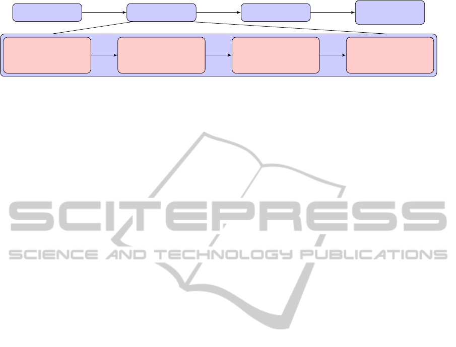
input image Φ
filter
segmentation
symbol-like
descriptors
1. smoothing
and dividing into
subwindows Ψ
i, j
2. compute distance
matrix ∆
i, j
and δ
m
i, j
3. apply threshold τ
4. accept smoothed
values or com-
pute weight ω
i, j
1. smoothing
and dividing into
subwindows Ψ
i, j
2. compute distance
matrix ∆
i, j
and δ
m
i, j
3. apply threshold τ
4. accept smoothed
values or com-
pute weight ω
i, j
Figure 1: Schematic of the proposed filter.
4. Computation and Updating of RGB Values.
At every iteration a global, image wide weight ω
i, j
is computed for normalization. A subwindow wide
weight, consisting of the squared distance of the user
based threshold τ and the pixelwise distance δ
r,s
, is
used for updating pixel values within one subwindow.
Please note that due to the sliding subwindows each
pixel gets updated N = k · l times. The global weight
ω
i, j
is initialized with zeros and updated according to
ω
i, j
←− ω
i, j
+ ψ
r,s
· (τ − δ
r,s
)
2
, (5)
where the ω
i, j
define the matrix Ω. For the updated
pixel values a third image frame Θ of the size of the
original image is needed. Θ is initalized with zeros
and updated according to
θ
θ
θ
i, j
←− θ
θ
θ
i, j
+ ψ
r,s
· (τ − δ
r,s
)
2
· ψ
ψ
ψ
m
. (6)
Again, every pixel value is updated N times. When
the algorithm has reached the last iteration, all up-
dated pixels Θ are added to the original image Φ and
normalized using Ω. Even though it is highly improb-
able that any entry in Ω equals zero, 1 is added to
every entry. As in general ω
i, j
0 and specifically
ω
i, j
≥ 0 is true, this does not change the outcome sig-
nificantly. This way the output is moved to the mean
color value ψ
ψ
ψ
m
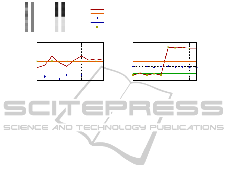
. Two examples for subwindow arrays
can be seen in figure 2(a) and 2(b) (grayscaled input
subwindow on the left side, output subwindow on the
right side). In figure 2(d) an example for noisy pix-
els in a subwindow is shown, which corresponds to
the image in 2(a). The pixelwise distance as well as
the mean pixelwise distance are below the threshold
τ, and the pixel color values are shifted towards the
mean color values. In figure 2(e) a noisy step func-
tion is shown, which relates to image 2(b). Here τ is
smaller than the distances and the pixels are not up-
dated to the mean value. Since we use sliding sub-
windows, the small scaled noise in pixels 0 to 4 and 5
to 9 will be corrected but the edge will be preserved.
2.2 Formulation of the Proposed Filter
in the Continuous Domain
Let f
f
f (x
x
x) define the smoothed input image, h
h
h(x
x
x) the
output image, c
c
c(ζ
ζ
ζ, x
x
x) measures the geometric close-
ness and s
s
s( f
f
f (ζ
ζ
ζ), f
f
f (x
x
x)) the photometric similarity. As
we want to address specifically color images, bold
letters refer to RGB-vectors. In this section | · | also
refers to per-element-multiplication instead of vector
multiplication. In our approach we first want to detect
noise and texture based on a user defined parameter τ.
If noise or texture is detected, we want to remove it,
and in case of a color edge, we want to preserve the
edge. Therefore, we define a mean value
m
m
m(x
x
x) = k
k
k
−1
m
(x
x
x)
Z
∞
−∞
Z
∞
−∞
f
f
f (ζ
ζ
ζ) · c
c
c(ζ
ζ
ζ, x
x
x)dζ
ζ
ζ
k
k
k
m
(x
x
x) =
Z
∞
−∞
Z
∞
−∞
c
c
c(ζ
ζ
ζ, x
x
x)dζ
ζ
ζ (7)
and a distance function
d ( f
f
f (x
x
x), m
m
m(x
x
x)) =
|
f
f
f (x
x
x) − m
m
m(x
x
x)
|
, (8)
which results in the pixelwise distance. The mean
value m
m
m(x
x
x) now holds the average color value inside
a spatial neighborhood of x
x
x and d holds the color dis-
tance from the pixel to the average m
m
m(x
x
x). If the spatial
neighborhood holds only small scaled noise or tex-
ture we expect a low pixelwise distance d, as well as
a low average pixelwise distance in the spatial neigh-
borhood c
c
c:
p(x
x
x) = k
−1
p
ZZ
∞
−∞
d ( f
f
f (ζ
ζ
ζ), m
m
m(x
x
x))c
c
c(ζ
ζ
ζ, x
x
x)dζ
ζ
ζ
k
p
(x
x
x) =
ZZ
∞
−∞
c
c
c(ζ
ζ
ζ, x
x
x)dζ
ζ
ζ. (9)
Therefore, we can make a binary decision using a
threshold τ as
h
h
h(x
x
x) = k
k
k
−1
R
(x
x
x) ·
(
RR
∞
−∞
f
f
f (ζ
ζ
ζ) · c
c
c(ζ
ζ
ζ, x
x
x) · s
s
s(ζ
ζ
ζ, x
x
x)dζ
ζ
ζ p, d ≤ τ
RR
∞
−∞
f
f
f (ζ
ζ
ζ) · c
c
c(ζ
ζ
ζ, x
x
x)dζ
ζ
ζ else,
(10)
where k
R
is the respective normalization. We used a
2D step function
c
c
c(ζ
ζ
ζ, x
x
x) =
(
1 x
x
x − a
a
a ≤ ζ
ζ
ζ ≤ x
x
x + b
b
b
0 else
, (11)
using the conditions a
a
a, b
b
b, e
e
e ∈ R
2
≥0
|a
a
a + b
b
b = e
e
e with a
fixed e
e
e. This generates a rectangle of the size e
e
e around
x
x
x. As this definition is not feasable in the continuous
ANovelReal-timeEdge-PreservingSmoothingFilter
7
(a) (b)
threshold τ
pixel color value ψ
r,s
mean pixel color value
pixelwise color distance δ
r,s
mean pixelwise color distance δ
m
Output Values
0
5
10
15
20
25
30
0 1 2 3 4 5 6 7 8 9
grayscale value
pixel number
(d)
0
20
40
60
80
100
0 1 2 3 4 5 6 7 8 9
grayscale value
pixel number
(e)
Figure 2: 2(a) Low level white noise (left) in 10 pixels is used as input for filtering. The right bar shows the same 10 pixels
after filtering. The computational steps involved in this image can be seen in figure 2(d). 2(b) A noisy step function is used
for input. After filtering input and output are indentical to preserve the edge. The computational steps are shown in figure
2(e). 2(d) The pixelwise and mean pixelwise distance are both below the threshold τ. The output is filtered according to (4)
and moved to the mean color. 2(e) The pixelwise and mean pixelwise distance are above the threshold and the output is not
filtered. The edge is therefore preserved.
domain as it generates a nonfinite number of subwin-
dows to calculte, in the discrete case however every
pixel is checked and updated according to its neigh-
borhood e
e
e. As a measure for similarity we used a
squared distance
s
s
s(x
x
x) = (τ − d( f
f
f (x
x
x), m
m
m(x
x
x)))
2
|m
m
m(x
x
x)| (12)
and the euclidian norm. In case of texture detection
the output is moved to the mean. The maximum size
of the step can be adjusted via the threshold τ.
2.3 Real-time Implementation
Real time can only be achieved by running the pro-
posed technique on parallel hardware, because the
computation of multiple subwindows is very inten-
sive on traditional CPUs. Once the image Φ is read,
values for the subwindows Ψ can be computed inde-
pendently. For accelaration we use a graphics pro-
cessor unit (GPU) and an example implementation
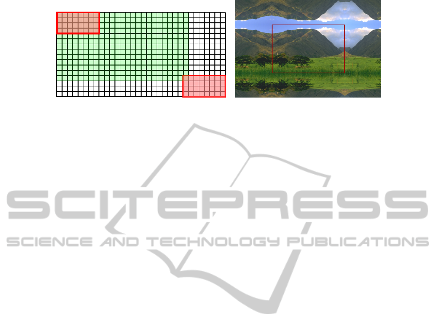
can be seen in figure 3(a). One block on the GPU
starts 32 × 16, and each of them loads one pixel into
shared memory. Each thread calculates the pixelwise
distances for one subwindow Ψ (marked red for two
example threads). As shown in white several threads
remain idle after copying. Since we are interested in
the average noise, we chose periodic mirrored bound-
ary conditions, which is illustrated in figure 3(b).
In our approach the images are filtered twice us-
ing subwindows of size k = 8, l = 4 and k = 4, l = 8.
Two runs are used for symmetry purposes and better
filter results. As ∆ and δ
m
are calculated over each
subwindow, this also sets the maximum size of tex-
ture that is detected. We tested two implementations
of the algorithm: The CPU measurement refers to a
single-threaded implementation using an AMD Phe-
nom 9550 quad-core processor at 2,2 GHz using one
core and 4 GB RAM. The GPU version is executed on
an Nvidia GTX580 graphics card using 512 cores and
1.5 GB device memory.
3 EXPERIMENTAL RESULTS
3.1 Filter Results
In figure 5 a visual comparison of different threshold
levels is shown. Above a threshold of τ = 35 the out-
put does not change much, which is easily understood
when looking at equation 4. Above a certain threshold
level every pixel is identified as either noise or texture
and smoothed out. Therefore, it is not necessary to
adapt the user based threshold τ to different noise lev-
els. As shown below, there is a best value for τ for
non-artificial images.
Also in this work noise and texture is treated
equally. But contrary to a denoising filter we do not
want to restore a noisy image, but fill out large ar-
eas with small color variations using the mean color.
This includes that noise, but also larger structures like
VISAPP2013-InternationalConferenceonComputerVisionTheoryandApplications
8
10 15 20 25 30
1
5
10
15
1
5
(a) (b)
Figure 3: 3(a) Example for parallelization on a GPU. One block loads 32 ×16px into shared memory where each subwindow,
shown in red, is computed by one thread. The next block would start at pixel 26. For the green pixels the weight ω will be
updated. 3(b) We used periodic mirrored boundary conditions as it leads to a good representation of the average noise at the
border.
texture, are smoothed out. As we are interested in
the perception-action loop of robots and improvement
of color-based segmentation results, the latter one is
more important to the results.
In figure 4(a) we compare the proposed filter to
a bilateral filter (Tomasi and Manduchi, 1998). As a
bilateral filter only smoothes the image based on the
spatial and color distance, it either does not preserve
the edge, but smoothes the texture, or preserves the
edge and does not filter the texture.
3.2 Segmentation Results
We filtered all images from the Berkeley Segmenta-
tion Dataset and Benchmark (Martin et al., 2001) us-
ing a large variety of different thresholds. Afterwards
the filtered images were segmented and compared
with the ground truth images from the database. The
performance was evaluated using the precision and re-
call method following (Martin et al., 2004). Given an
original image Φ, its machine segmentation S
0
, and
the corresponding ground truth S, precision is defined
as the fraction of boundary pixels in the segmented
image S
0
that also occur in the ground truth S over
the total number of boundary pixels in S
0
. It is there-
fore sensitive to over-segmentation. Recall measures
the fraction of boundary pixels in S which are also
found in S
0
. It is sensitive to under-segmentation. The
results shown are the arithmetic means of all values
computed.
Figure 6(a) shows the precision and recall val-
ues for the Metropolis algorithm using constant seg-
mentation parameters for various threshold values τ.
Above a threshold of τ = 35 the values remain steady.
The weighted mean of precision and recall indicate
that best results are obtained for a threshold of τ = 30.
This behavior was also observed using different seg-
mentation parameters and may also be seen in the
filtered images shown in figure 5. Also note that
precision is considerably lower than recall. While
the ideal value would be 1 for both, the segmented
images are extremely rich on texture, resulting in
over-segmentation. The threshold is computed using
the Berkeley Segmentation Dataset and Benchmark
which offers a wide range of heavily textured natural
images. However, our experiments show that τ = 30
may be considered a good value for all scenes offer-
ing good color contrast. As in low contrast scenes the
color segmentation will most likely fail, we do not
take it into further consideration.
In figure 6(b) we show the segmentations for dif-
ferent values of the parameter α
1
using the Metropo-
lis algorithm. The parameter α
1
is a system parame-
ter used to increase or decrease the coupling strength
in the clustering model. Thus, it influences the total
number of segments. Other parameters were taken
from (Abramov et al., 2012). Best results in the
trade-off between over- and under-segmentation were
achieved for α
1
= 1.0.
Next, we compare our method with the graph-
based segmentation, mean-shift algorithm and an al-
ternative version of the Metropolis algorithm using
the standard bilateral filter for smoothing (see figure
6(c)). While the Metropolis algorithm without filter
performs better than the graph-based and mean shift
segmentation, precision is improved when using the
proposed filter. Results are shown for different α
1
values for the Metropolis algorithm. The value for
α
1
= 1.0 is marked with a circle. For graph-based
segmentation we used the combination of parameters
recommended by the authors for segmentation of ar-
bitrary images, see (Felzenszwalb and Huttenlocher,
2004). The mean shift algorithm of (Paris and Du-
rand, 2007) uses three input parameters: the Gaus-
sian parameters σ
c
and σ
s
for color and spatial do-
main respectively and the persistent threshold τ
p
. We
determined experimentally the combination σ
c
= 2,
σ
s
= 8 and τ
p
= 1 for best results. On purpose, we
ANovelReal-timeEdge-PreservingSmoothingFilter
9
(a) (b) (c)
0
100
200
0 100 200 300 400
color value
pixel nr
r
g
b
(d)
0
100
200
0 100 200 300 400
color value
pixel nr
r
g
b
(e)
0
100
200
0 100 200 300 400
color value
pixel nr
r
g
b
(f)
Figure 4: 4(a) Artificial input image with three features: a green color edge, texture is simulated using red squares 7px wide,
and white noise is added. A cross section is shown in white and can be seen in figure 4(d). 4(b) Bilateral Filter. For an
arbitrary large kernel of 20 px in the space domain and using σ
c
= 200 for the color domain all texture and noise is filtered.
The color edge now has a width of 18 px. A cross section can be seen in figure 4(e). 4(c) Proposed texture filter. The edge
remains sharp and all texture, as well as noise is smoothed out. A cross section can be seen in figure 4(f). 4(d) Cross section
of original image. A green color step, as well as texture and noise can be seen. 4(e) Cross section of the bilateral filter. The
color edge is not preserved, texture is removed, but some noise remains. 4(f) Cross section of proposed filter. The green color
edge is preserved and texture, as well as all noise is removed.
Figure 5: Effect of different thresholds. For low thresholds the image is more blurred, after τ = 30 it does not change much.
From top left to bottom right: τ = 5, 20, 30, 40, 60, 80.
did not combine the mean-shift and the graph-based
algorithm with the proposed filter, because both algo-
rithms already perform their own preprocessing.
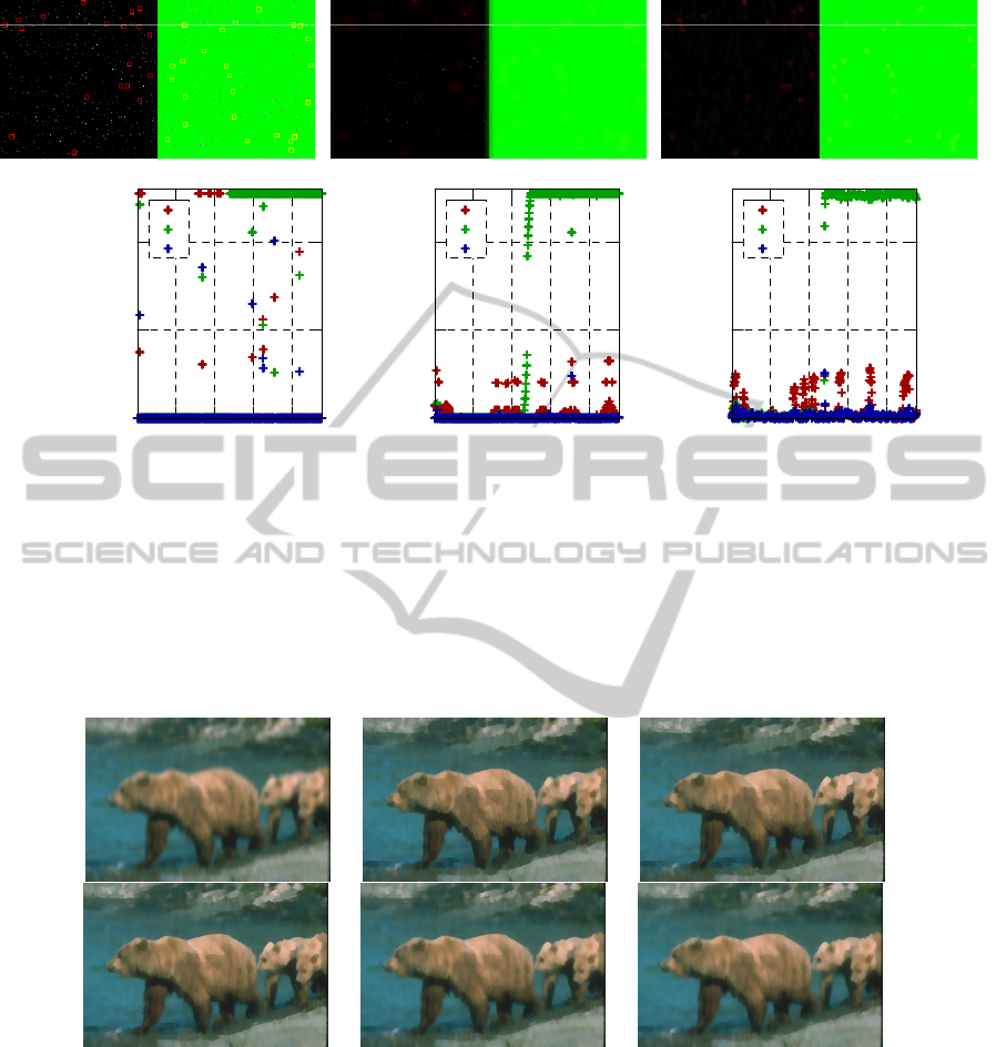
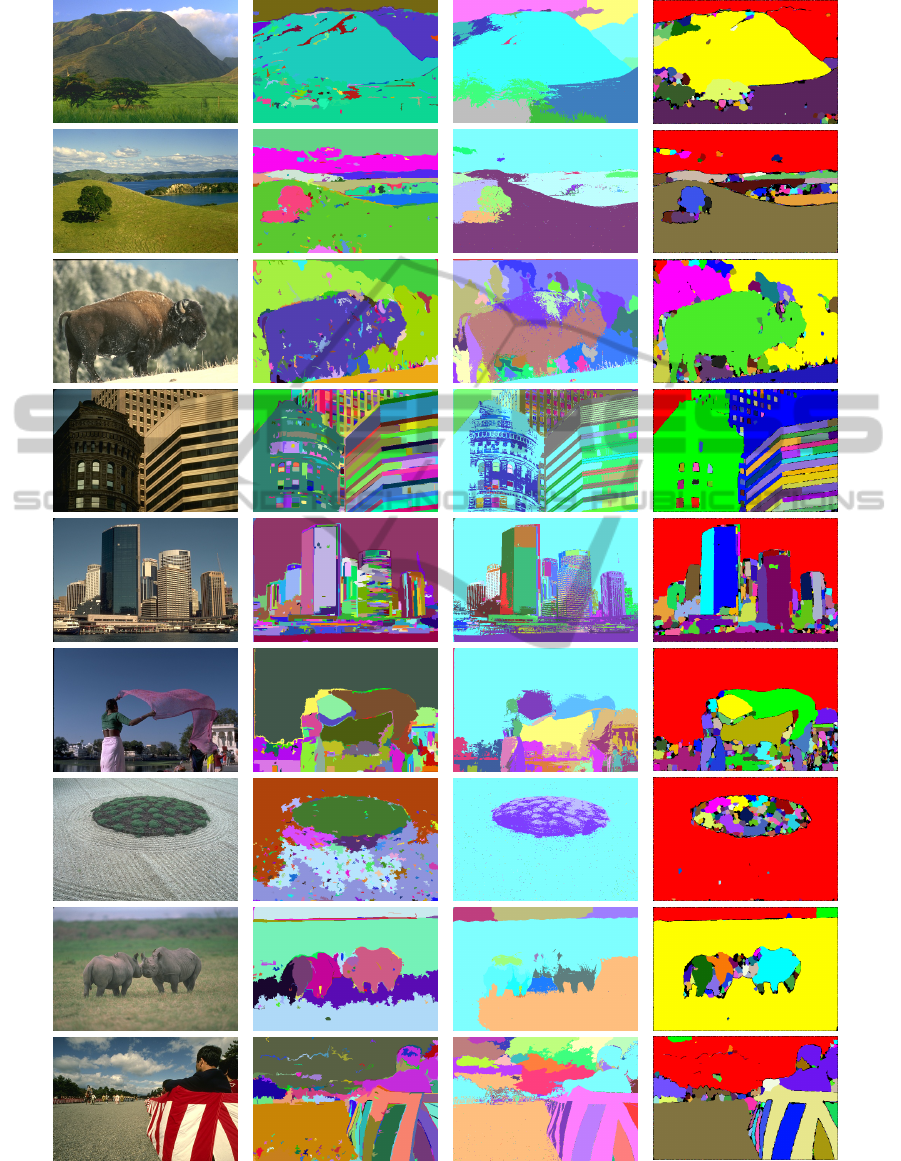
A visual comparison can be seen in figure 7. The
proposed filter greatly reduces noise and texture and
achieves a good trade-off between over- and under-
segmentation as compared to the other methods. A
comparison for a video sequence using the metropo-
lis algorithm may be seen in figure 8. Labels are kept
during the sequence and are encoded using different
colors: both mean-shift and graph based segmenta-
tion do not use fixed label numbers for objects. The
filter reduces the over-segmentation in textured areas,
e.g. the suitcases, the pad, or the plant.
For robotic applications it is very important that
the labels of image segments do not change through-
out a video stream. Currently only very few segmen-
tation algorithms running in real-time do achieve this
(Abramov, 2012), among them the Metropolis algo-
rithm.
VISAPP2013-InternationalConferenceonComputerVisionTheoryandApplications
10

0,2
0,4
0,6
0,8
1
0 20 40 60 80
precision / recall
Threshold τ
precision
recall
(a)
0,4
0,5
0,6
0,7
0,8
0,9
1
0,28 0,32 0,36 0,4
recall
precision
α
1
= 0.8
α
1
= 0.9
α
1
= 1.0
α
1
= 1.1
α
1
= 1.2
α
1
= 2.0
(b)
0,5
0,6
0,7
0,8
0,9
1
0,2 0,25 0,3 0,35 0,4
recall
precision
metropolis without filter
metropolis with bilateral filter
metropolis with proposed filter
graph-based
mean shift
(c)
Figure 6: 6(a) Metropolis algorithm performance with fixed parameters using filtered images for various thresholds. 6(b)
Estimating best segmentation parameters for a fixed threshold τ = 30 using filtered images. 6(c) Comparison between graph-
based, mean shift and Metropolis algorithm. Metropolis segmentation using α
1
= 1.0 is marked with a circle.
3.3 Time Performance Results
We computed the average frame rates for images of
different sizes in table 1. For comparison purposes,
images from the Berkeley Segmentation Dataset and
Benchmark were used (Martin et al., 2001). As
shown in section 2 the complexity is independent of
the threshold used. You can see that the GPU ver-
sion is roughly 30 times faster than the CPU ap-
proach, independent of the image size. For images
of size 480 ×320 px real-time processing of movies is
achieved.
Table 1: Time performance for images of different sizes.
The test image was taken from the training set of the Berke-
ley Segmentation Dataset and Benchmark (Martin et al.,
2001) and is also used in figure 3(b). 100 measurements
were taken and averaged.
Image Size CPU GPU
[px] [Hz] [s] [Hz] [ms]
240 × 180 3.03 0.33 80.38 12.4
320 × 240 1.66 0.60 48.00 20.8
480 × 320 0.80 1.25 23.81 42.0
640 × 480 0.40 2.50 12.35 81.0
800 × 600 0.24 4.17 7.65 130.7
1024 × 768 0.15 6.67 4.24 235.9
4 CONCLUSIONS
In this paper, we presented a novel real-time edge
preserving smoothing filter, which replaces noisy and
textured areas by uniformly colored patches. The
performance of a recent image segmentation method
could be significantly improved using the filtered im-
ages. The time performance makes the filter applica-
ble to video streams, as shown in figure 8, and hence
can be used in the future as a component inside the
perception-action loop of robotic applications. The
proposed method improves the precision and recall
trade-off of obtained segmentations. Furthermore, the
detected features could be used for classification pur-
poses in other applications.
ACKNOWLEDGEMENTS
The research leading to these results has received
funding from the European Community’s Seventh
Framework Programme FP7/2007-2013 (Specific
Programme Cooperation, Theme 3, Information and
Communication Technologies) under grant agree-
ment no. 269959, Intellact. B. Dellen acknowledges
support from the Spanish Ministry of Science and In-
novation through a Ramon y Cajal program.
ANovelReal-timeEdge-PreservingSmoothingFilter
11
(a) (b) (c)
(d)
Figure 7: Visual comparison of several threshold levels. 7(a) Original image. 7(b) Graph based segmentation. 7(c) Mean-shift
segmentation. 7(d) Proposed filter in connection with metropolis algorithm.
VISAPP2013-InternationalConferenceonComputerVisionTheoryandApplications
12
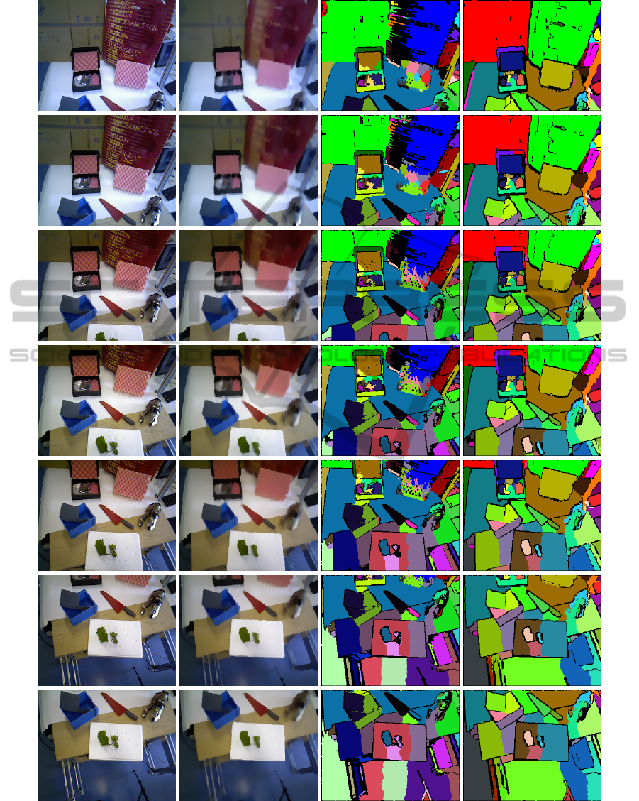
(a) (b) (c) (d)
Figure 8: Visual comparison of a short video sequence. 8(a) Original frames from sequence. 8(b) Filtered frames from
sequence using the proposed filter. 8(c) Segmentation using the Metropolis algorithm without filter. 8(d) Segmentation using
the Metropolis algorithm and the proposed filter. There is significant less over-segmentation in textured areas (e.g. suitcase,
pad).
ANovelReal-timeEdge-PreservingSmoothingFilter
13

REFERENCES
Abramov, A. (2012). Compression of the visual data
into symbol-like descriptors in terms of the cognitive
real-time vision system. PhD thesis, Georg-August-
Universität Göttingen.
Abramov, A., Pauwels, K., Papon, J., Wörgötter, F., and
Dellen, B. (2012). Real-time segmentation of stereo
videos on a portable system with a mobile gpu. IEEE
Transactions on Circuits and Systems for Video Tech-
nology.
Cigla, C. and Aydin Alatan, A. (2008). Depth assisted ob-
ject segmentation in multi-view video. In 3DTV Con-
ference: The True Vision - Capture, Transmission and
Display of 3D Video, 2008, pages 185 –188.
Comaniciu, D. and Meer, P. (2002). Mean shift: a robust
approach toward feature space analysis. IEEE Trans-
actions on Pattern Analysis and Machine Intelligence,
24(5):603 –619.
Du, W., Tian, X., and Sun, Y. (2011). A dynamic threshold
edge-preserving smoothing segmentation algorithm
for anterior chamber oct images based on modified
histogram. In 4th International Congress on Image
and Signal Processing (CISP), volume 2, pages 1123
–1126.
Durand, F. and Dorsey, J. (2002). Fast bilateral filtering
for the display of high-dynamic-range images. ACM
Trans. Graph., 21(3):257–266.
Elad, M. (2002). On the origin of the bilateral filter and
ways to improve it. IEEE Transactions on Image Pro-
cessing, 11(10):1141 – 1151.
Farbman, Z., Fattal, R., Lischinski, D., and Szeliski, R.
(2008). Edge-preserving decompositions for multi-
scale tone and detail manipulation. ACM Trans.
Graph., 27(3):67:1–67:10.
Farmer, M. and Jain, A. (2005). A wrapper-based approach
to image segmentation and classification. IEEE Trans-
actions on Image Processing, 14(12):2060 –2072.
Farsiu, S., Elad, M., and Milanfar, P. (2006). Multiframe de-
mosaicing and super-resolution of color images. IEEE
Transactions on Image Processing, 15(1):141 –159.
Felzenszwalb, P. and Huttenlocher, D. (2004). Efficient
graph-based image segmentation. International Jour-
nal of Computer Vision, 59:167–181.
Jiang, W., Baker, M. L., Wu, Q., Bajaj, C., and Chiu, W.
(2003). Applications of a bilateral denoising filter in
biological electron microscopy. Journal of Structural
Biology, 144(1–2):114 – 122.
Lev, A., Zucker, S. W., and Rosenfeld, A. (1977). Iterative
enhancemnent of noisy images. IEEE Transactions on
Systems, Man and Cybernetics, 7(6):435 –442.
Martin, D., Fowlkes, C., and Malik, J. (2004). Learning
to detect natural image boundaries using local bright-
ness, color, and texture cues. IEEE Transactions on
Pattern Analysis and Machine Intelligence, 26(5):530
–549.
Martin, D., Fowlkes, C., Tal, D., and Malik, J. (2001).
A database of human segmented natural images and
its application to evaluating segmentation algorithms
and measuring ecological statistics. In Proc. 8th Int’l
Conf. Computer Vision, volume 2, pages 416–423.
Muneyasu, M., Maeda, T., Yako, T., and Hinamoto, T.
(1995). A realization of edge-preserving smoothing
filters using layered neural networks. In IEEE Interna-
tional Conference on Neural Networks, Proceedings.,
volume 4, pages 1903 –1906 vol.4.
Paris, S. and Durand, F. (2007). A topological approach to
hierarchical segmentation using mean shift. In IEEE
Conference on Computer Vision and Pattern Recogni-
tion (CVPR), pages 1 –8.
R., R. and W., S. (2003). Adaptive demosaicking. J. Elec-
tron. Imaging, 12(12):633.
Sun, D., Roth, S., and Black, M. (2010). Secrets of optical
flow estimation and their principles. In IEEE Con-
ference on Computer Vision and Pattern Recognition
(CVPR), pages 2432 –2439.
Tomasi, C. and Manduchi, R. (1998). Bilateral filtering for
gray and color images. In Sixth International Confer-
ence on Computer Vision, pages 839 –846.
Xiao, J., Cheng, H., Sawhney, H., Rao, C., and Isnardi,
M. (2006). Bilateral filtering-based optical flow es-
timation with occlusion detection. In Leonardis, A.,
Bischof, H., and Pinz, A., editors, Computer Vision –
ECCV 2006, volume 3951 of Lecture Notes in Com-
puter Science, pages 211–224. Springer Berlin / Hei-
delberg.
Yang, Q., Wang, S., and Ahuja, N. (2010). Svm for edge-
preserving filtering. In IEEE Conference on Computer
Vision and Pattern Recognition (CVPR), pages 1775 –
1782.
VISAPP2013-InternationalConferenceonComputerVisionTheoryandApplications
14
