
An Image Segmentation Assessment Tool ISAT 1.0
Anton Mazhurin
1
and Nawwaf Kharma
2
1
ALMAZ Technology, 1790 du Canal, 302, Montreal (QC), H3K 3E6, Canada
2
Department of Electrical & Computer Engineering, Concordia University, Montreal (QC), H3G 1M8, Canada
Keywords: Image Segmentation, Quality Assessment, Software Tool, Pixel-based Measures, Region-based Measures.
Abstract: This paper presents algorithms and their software implementation, which assess the quality of segmentation
of any image, given an ideal segmentation (or ground truth image) and a usually less-than-ideal
segmentation result (or machine segmented image). The software first identifies every region in both the
ground truth and machine segmented images, establishes as much correspondence as possible between the
images, then computes two sets of measures of quality: one, region-based and the other, pixel-based. The
paper describes the algorithms used to assess quality of segmentation and presents results of the application
of the software to images from the Berkeley Segmentation Dataset. The software, which is freely available
for download, facilitates R&D work in image segmentation, as it provides a tool for assessing the results of
any image segmentation algorithm, allowing developers of such algorithms to focus their energies on
solving the segmentation problem, and enabling them to tests large sets of images, swiftly and reliably.
1 MOTIVATION & REVIEW
Many researchers develop, extend and apply
algorithms for image segmentation. A natural part of
their work is the assessment of the quality of the
results achieved by the segmentation algorithm.
Most day-to-day assessment work, during the
development stage is done by eye, with more
rigorous computerized evaluations carried out
towards the end of the development cycle, using in-
house scripts or programs that are almost always
pixel-based, and still require a fair amount of manual
labelling. Now, this may be acceptable if the entity
doing the development is human, but is impossible if
one intends to utilize an automated method for
image segmentation program development, such as
genetic programming (Singh, 2009).
Hence, for reasons of (a) freeing researchers and
developers from the task of building their own
image segmentation quality assessment tool; (b)
providing the community with not just pixel-based
but also region-based measures that (c) do not
require manual labelling of the various regions of
the image, and in a package that (d) can provide an
objective function for automated development
applications, for all the above reasons, we have
specified and developed ISAT 1.0.
In the literature, there is hardly any immediately
usable software tools dedicated to the automated
assessment of mage segmentation results, from both
pixel- and region-based perspectives, a tool that only
requires edge-images of the machine segmented
result and the human generated ground truth, and
without any need for region marking.
There are, however, a large number of related
publications worthy of note. They include the work
by (Francisco, 2009), (Jiang, 2006), (Cardoso, 2005)
and most recently, (McGuiness, 2011). These and
others use approaches that all come under two
mutually exclusive categories: objective evaluation
methods that do not involve a human operator and
subjective assessment methods that do (Zhang,
2008). Of the objective evaluation methods, only
empirical methods assess the quality of
segmentation by direct evaluation of the resulting
segmented images, and they do so in either
supervised or unsupervised ways. Unsupervised
means of segmentation quality evaluation do not
require a ground truth image, but decide the quality
of segmentation based on the presence of certain
characteristics normally associated with properly
segmented images (Unnikrishnan, 2007). These
methods have their advantages, as they allow
automated evaluation of a large number of
segmented images without the laborious effort
needed for manual production of a large number of
436
Mazhurin A. and Kharma N..
An Image Segmentation Assessment Tool ISAT 1.0.
DOI: 10.5220/0004216404360443
In Proceedings of the International Conference on Computer Vision Theory and Applications (VISAPP-2013), pages 436-443
ISBN: 978-989-8565-47-1
Copyright
c
2013 SCITEPRESS (Science and Technology Publications, Lda.)

matching ground truth images. However, it is well-
known that that such an approach will often fail
under conditions where the required segmentation is
related to the meaning of the segmented image.
Indeed, if a reliable unsupervised objective method
had existed then it would have formed the basis of
one of the best (if not the best) image segmentation
algorithms to date. That is not the case. Hence,
researchers still utilize either subjective evaluation,
which requires ground truth or supervised objective
evaluation, which also requires ground truth. Our
method comes under supervised means of objective
evaluation, and it is assessed – as it ought to be – by
subjective visual inspection.
2 METHODOLOGY
ISAT assesses the quality of segmentation of any
image. To do so, ISAT does not require the original
image, but two other images representing the ideal
and actual segmentation of the original image. As a
matter of terminology, the ideally segmented image,
which is usually drawn by hand, is called the ground
truth image (or GT). The other image represents the
result of a segmentation procedure, which is usually
executed by machine, and is called the Machine
Segmented image (or MS). Both of these images are
binary images, in that they exhibit the boundaries of
the segmented regions as black curves on a white
background. In all following calculations, it is the
GT that functions as a reference of presumed truth
against which a MS image is judged.
To carry out any kind of segmentation quality
assessment, connected regions in both GT and MS
images must be established then, crucially, every
region in GT must – if possible – be matched with
one or more regions in MS. Note that one region in
GT may match one region in MS; that region in GT
would then be correctly segmented if the overlap
between the two regions is great enough or missed if
the overlap is insufficient. Also, more than one
region in GT may be matched with one region in
MS; that region in GT would be under-segmented.
On the other hand, multiple regions in MS may
correspond to one region in GT; that region in GT
would then be over-segmented. Finally, every region
that exists in MS but does not correspond to any
region(s) in GT is considered noise. Region-based
accuracy is calculated as a ratio of the number of
correctly matched regions in MS to the sum of all
the regions in GT, plus the number of noise regions
(which come from MS). All of the above measures
were based on equivalent measures proposed by
Hoover et al. (Hoover, 1996).
As such, an ideally segmented image, from a
region-based perspective, entails that every region in
GT is exclusively matched with exactly one region
in MS, with zero noise (i.e., unmatched regions in
MS). And in fact, ISAT will return a region-based
accuracy of 100%, for this case. Note that matching
requires an overlap between the two matched
regions exceeding a pre-set threshold, which we
currently set to 66% and should not be set to 100%.
This ensures that the number of correctly segmented
regions reflects human conceptions of region-based
segmentation, where the number of approximately
matched regions (e.g., red blood cells) matter more
than the precise fit of every matched region (e.g.,
one blood cell).
Once region identification in both GT and MS is
completed, and matching of regions between GT and
MS is done, it is possible to compute all region-
based segmentation quality measures. But also, this
makes it possible to compute the other set of pixel-
based segmentation quality measures. These
measures sound familiar, but they are applied
differently than the well-known True Positive, False
Negative, True Negative and False Positive
measures used in innumerable studies in image
processing (Bushberg, 2002). We will describe the
final pixel-based measures here intuitively, as the
following sub-sections describe all the measures, in
full detail. In brief, the final pixel-based measures
provide a normalized image-wide quantitative
assessment of the quality of the fit between the
regions of GT and those they were matched with in
MS. As such, our sensitivity is the percentage of
pixels of regions of GT that were matched with
regions in MS. Specificity is the percentage of pixels
of the backgrounds of the various regions in GT that
were in fact assigned to backgrounds of the
matching regions in MS. We define the background
of a region as those pixels that belong to the image
but not to that region, and we exclude the pixels of
the edges between regions from all calculations.
An ideally segmented image, from a pixel-based
perspective is similar to an ideally segmented image,
from a region-based point of view, but for one
exception. Using the red blood cells example, every
blood cell boundary in the MS image must fit
perfectly the boundary of every corresponding blood
cell in the GT image; any deviation no matter how
small will reduce either sensitivity or specificity and
hence the overall pixel-based measure of accuracy,
which is a weighted average of the two.
AnImageSegmentationAssessmentToolISAT1.0
437
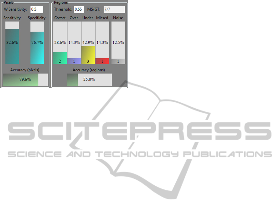
Figure 1: The results window in ISAT 1.0.
2.1 Region-based Measures
First, ISAT enumerates and marks all connected
regions in both GT and MS images. The number of
pixels in every region is also computed and stored.
The pixels that make-up the boundaries of the
regions are eliminated from the calculations, as they
do not belong to any region. Let N be the number of
regions in the GT image and M be the number of
regions in the MS image. Let the number of pixels in
each GT region R
n
be called P
n
(where n = 1... N).
Similarly, let the number of pixels in MS region R
m
be called P
m
(were m = 1… M). An overlap table
with size N×M is calculated. Every cell O
n,m
in the
overlap table contains the number of pixels in the
overlapping area of the two corresponding regions
R
n
and
R
m
. If the two regions do not overlap then the
value O
n,m
will be zero. If there is a perfect match
between the two regions then O
n,m
= P
n
= P
m
.
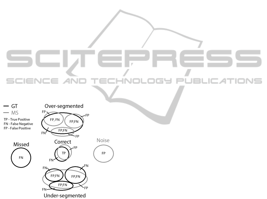
Second, a classification procedure marks every
region as a member of one of the five exclusive
groups: correct, over-segmented, under-segmented,
missed and noise. The classification procedure uses
a single input parameter threshold T. This parameter
defines the strictness of all group classifications; the
default value is 0.66 (~2/3). Classification rules for
every group follow (consult Figure 2).
Correct: GT region R
n
and MS region R
m
are
marked as correct IFF
(a) at least T percent of GT region R
n
overlaps
with region R
m
. This can be expressed as:
O
n,m
>= T . P
n
(1)
AND
(b) at least T percent of MS region R
m
overlaps
with region R
n
, formulaically expressed as:
O
n,m
>= T . P
m
(2)
Over-segmented: GT region R
n
and a set of MS
regions R
m1
… R
mx
(were 2 <= x <= M) are
marked over-segmented IFF
(a) for every MS region R
mi
in the set (where i =
1... x), at least T percent of that region overlaps
with GT region R
n
. Also, expressed as:
O
n,mi
>= T . P
mi
(3)
AND
(b) at least T percent of GT region R
n
overlaps
with the union of the set of MS regions. This is
expressed as:
x
∑O
n,mi
>= T . P
n
i=1
(4)
Under-segmented: MS region R
m
and a set of GT
regions R
n1
… R
nx
(were 2 <= x <= N) are
marked as under-segmented IFF
(a) for each GT region R
ni
in the set (where i =
1... x), at least T percent of that region overlaps
with MS region R
m.
This can be expressed as:
O
ni,m
>= T . P
ni
(5)
AND
(b) at least T percent of MS region R
m
overlaps
with the union of the set of GT regions, also
expressed as:
x
∑O
ni,m
>= T . P
m
i=1
(6)
Missed: a GT region R
n
is marked as missed if it
has not been marked as correct, over-segmented
or under-segmented.
Noise: a MS region R
m
is marked as noise if it
has not been marked as correct, over-segmented
or under-segmented.
After the regions are classified, we normalize the
numbers of regions in every group using the
following rules; this results in percentages.
for correct regions: the number of GT regions
marked as correct is divided by the total number
of GT regions.
for over-segmented regions: the number of GT
regions marked as over-segmented is divided by
the total number of GT regions.
for under-segmented: the number of GT regions
marked as under-segmented is divided by the
total number of GT regions.
VISAPP2013-InternationalConferenceonComputerVisionTheoryandApplications
438

for missed regions: the number of GT regions
marked as missed is divided by the total number
of GT regions.
However, for noise regions: the number of MS
regions marked as noise is divided by the sum of
(a) the number of MS regions marked as noise
plus (b) the total number of GT regions.
Figure 2: All possible classifications of regions in a GT
and corresponding MS image (if any).
The accuracy value of the region-based measures
(AccuracyR) is calculated as the ratio of number of
correct regions to the sum of (a) the total number of
GT regions and (b) the number of noise regions.
AccuracyR = NumCorrect / (N + NumNoise) (7)
N is the total number of GT regions;NumCorrect is
number of correct regions; NumNoise is the number
of noise regions.
2.2 Pixel-based Measures
For every match between one or more GT regions
with one or more MS regions, and for every GT and
MS region that is un-matched, four basic values are
computed (some returning zero values): True
Positive (TP), False Negative (FN), True Negative
(TN) and False Positive (FP). This results in
individual results that must be summed up, before
image-wide overall TP, FN, TN and FP can be
calculated.
In more detail (see Figure 3), one GT region
could match exactly one MS region (giving us a
‘correct’ group); one GT region could match more
than one MS region (giving us an ‘over-segmented’
group of pixels) and conversely one MS region
could match more than one GT region (giving us an
‘under-segmented’ group of pixels). Finally, there
are regions in GT that are not matched with any MS
region (the ‘missed’ group) and MS regions that are
not matched with any GT regions (the ‘noise’
group). It is important to underline the fact that the
following calculations provide us with a whole set of
TP, FN, TN and FP numbers that must be summed
up, before overall image-wide figures for TP, FN,
TN and FP can be secured. It is those overall values
that are used to compute specificity and sensitivity,
then pixel-based accuracy.
So, to begin with, for every matched and un-
matched region in GT and MS, the following
individual TP, FN, TN and FP values are computed,
according to the following rules.
True Positive. TP relies on one source:
(a) Correct group: the number of pixels in the
overlap area of GT region R
n
and MS region R
m
.
TP = O
n,m
(8)
False Negative. FN comprises the number of
pixels from four different groups:
(a) Correct group: the number of pixels in GT
region R
n
which are not in an overlap area with
MS region R
m
.
FN
correc
t
= P
n
- O
n,m
(9)
(b) Other groups, comprising of over-segmented,
under-segmented and missed groups. This is the
number of pixels in GT regions.
FN
othe
r
= P
n
(10)
FN is the sum of FN
correct
and
FN
other
.
True Negative. TN relies on one source, but
involves a necessary normalization.
(a) Correct group: the calculation is performed in
two steps in order to avoid dependence on image
dimensions. First, the normalized value TN
norm
is
calculated as a ratio of (a) the number of actual
TN pixels (the number of pixels in the image
which are not in GT region R
n
AND not in MS
region R
m
) to (b) the maximum possible number
of TN pixels for this region (equals the number
of pixels in the image which are not in GT region
R
n
). This is expressed as:
TN
norm
= (N
total
– (P
n
+ P
m
– O
n,m
)) / (N
total
- P
n
)
(11)
Note that N
total
is the number of pixels in the
image. Second, the value of TN
norm
is weighted
by the number of pixels in GT region R
n
:
TN = TN
norm
. P
n
(12)
AnImageSegmentationAssessmentToolISAT1.0
439
False Positive. FP comprises the total number of
pixels belonging to four groups:
(a) Correct group: the calculation is performed in
two steps in order to reflect the normalization of
the complimentary value of TN (see (11) and
(12)). First, the normalized value FP
norm
is
calculated as a ratio of (a) the number of actual
FP pixels (the number of pixels in MS region R
m
which are not in the overlap area with GT region
R
n
) to (b) the maximum possible number of FP
pixels for this region (the number of pixels in
MS region R
m
).
FP
norm
= (P
m
- O
n,m
) / P
m
(13)
Second, the value of FP
norm
is weighted by the
number of pixels in GT region R
n
:
FP
correc
t
= FP
norm
. P
n
(14)
(b) Other groups, comprising of over-segmented,
under-segmented and noise groups. This is the
number of pixels in MS regions.
FP
othe
r
= P
m
(15)
FP is the sum of FP
correct
and
FP
other
.
Figure 3: All possible classifications (except
TrueNegative) of pixels in an MS region, relative to its
corresponding GT regions.
As stated above, once all four values are calculated
for the various matched and unmatched regions in
GT and MS, the individual TP, FP, TN and FP
figures are summed up, and the resulting Overall
TP, Overall FP, Overall TN and Overall FP values
are used in the formulas to calculate sensitivity,
specificity and accuracy. Note that W
sens
is the
weight assigned to sensitivity, which takes a value in
the range of [0,1] with its default set to 0.5.
Sensitivity = (Overall TP) / (Overall TP +
Overall FN)
(16)
Specificity = (Overall TN) / (Overall TN +
Overall FP)
(17)
AccuracyP = W
sens
. Sensitivity +
(1 – W
sens
) . Specificity
(18)
3 APPLICATION NOTE
ISAT 1.0 installation package for Win32 platform is
currently available for free download at
www.ece.concordia.ca/~kharma/ExchangeWeb/ISA.
The package is a fully functional application
with a GUI. It can be used in various image
segmentation tasks as is. Additionally, it has C++
and C# APIs that allow for its use as a library, by
other programs.
The user has to specify three folders for Original
images, GT images and MS images. ISAT
enumerates all the images in the folder, and it
automatically matches Original, GT and MS images
using a simple rule: the names of both GT and MS
image files have as prefix the name of the
corresponding original image file. The installation
package contains a set of sample images.
ISAT displays all three images (original, GT and
MS) in a single window on top of each other, and
enables control of the opacity of every image for
visual evaluation of segmentation quality.
ISAT supports all major image formats and is
also able to read the special ‘.seg’ file format used
by the Berkeley Segmentation Dataset and
Benchmark or BSDB (Berkeley, 2012).
4 RESULTS
To evaluate our methodology through the
application of ISAT 1.0, we make use of the well-
known Berkley Segmentation Dataset and
Benchmark picked a few examples to exhibit how
well the results reflect human conceptions of
segmentation quality, within bounds of theoretical
correctness. By that, we mean (a) MS images that
generate ideal or near-ideal segmentation results
should give perfect or near-perfect accuracy results,
respectively; (b) MS images that exhibit over-
segmented or under-segmented regions should
respectively have over- and under-segmentation
results that reflect that fact; (c) MS images that
identify non-existing regions or miss some regions
VISAPP2013-InternationalConferenceonComputerVisionTheoryandApplications
440
in GT altogether, should have that noted in elevated
missed and noise values. In addition, (d) images
with identical region-based measures that differ –
even a little – in precision of fit, between MS and
corresponding GT regions, should have different
pixel-based measurement values.
The first example is shown in Figure 4. The first
row has the original image on the left and the GT
image on the right. The first MS image is the second
one from the top. It obviously is greatly under-
segmented and is missing a large number of GT
regions, but suffering little noise. This is reflected in
the measures on the left-hand side, as under-
segmentation is at 65.2% while over-segmentation is
zero, correctly identified regions is low at 6.1%
while 28.8% of GT regions were completely missed.
This MS image gives an overall region-based
accuracy of 5.8% and a larger pixel-based accuracy
of 41.4% (due to the large size of the four regions
that were correctly segmented). Going down the
right column, we see another MS image with well-
identified petals and nothing else, taking down
region-based accuracy to 2 regions (or 3%) and
reducing pixel-based accuracy to 38%. This is
followed by the last MS image with a deservedly
low pixel-based accuracy of just 17.6%.
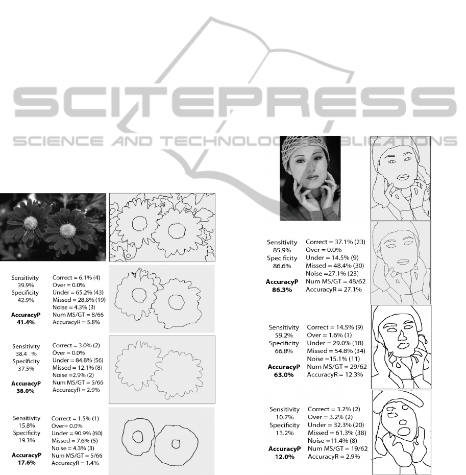
Figure 4: The original image of two flowers (BSDB
training image #124084) and the ground truth image,
followed by three segmentation results with decreasing
levels of quality.
The second example shows the face of a woman.
Again, the first row has on the left the original
image, which does not enter into processing, and on
the right the ideal or GT image. Each of the second,
third and fourth rows have on the right an MS image
and on the left the results of comparing that image to
the GT using ISAT. It is clear to the naked eye that
the quality of segmentation decreases from top to
bottom. The first segmentation result (second row) is
almost as good as the GT, except that it under-
segments and misses altogether a few regions that
appear in GT; it also introduces regions that have no
equivalent in GT. This reflects itself in a significant
under-segmentation score of 14.5% and high values
for both missed (48.4%) and noise (27.1%) measures
of region-based segmentation quality. All in all,
region-based accuracy is 27.1%, as only 23 of the
GT’s 62 regions were correctly matched. On the
pixel-based front, sensitivity and specificity for the
higher figures are higher (at 86.3% and 63% vs. 12%
for the lowest MS).
Figure 5: The original image of a woman (BSDB training
image# 302003) and the ground truth image, followed by
three segmentation results with decreasing levels of
quality.
AnImageSegmentationAssessmentToolISAT1.0
441
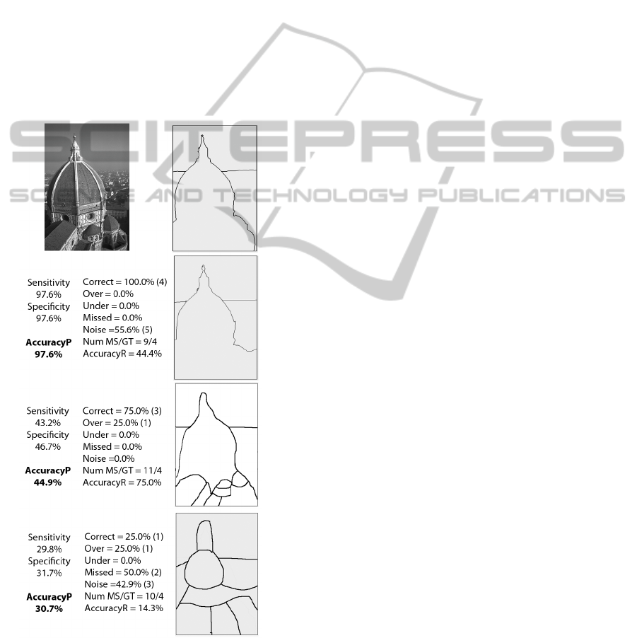
Figure 6 presents a structure, with a rather simplified
ideal or GT image. As with the preceding examples,
the first row contains the original image (left) and
the ideal segmentation (right). The other rows have
an MS image (right) next to the segmentation quality
data (left) coming from ISAT’s comparison of the
MS image to the GT image. The first result in the
second row shows what appears to be near-perfect
segmentation, yielding a pixel-based accuracy of
97.6%. Closer inspection, however, reveals a
number (5) of tiny regions in the MS image that do
not correspond to any regions in GT. This is the
reason for the elevated noise value of 55.6% and
hence low region-based accuracy of 44.4%. Skirting
that anomaly, correctness returns a value of 100%,
as all regions in GT have matching regions in the
MS image.
Figure 6: The original image of a structure (BSDB training
image #24004) and the ground truth image, followed by
three segmentation results with decreasing levels of
quality.
Going down to the third row in Figure 6, one can
identify a few regions in the MS image, which do
not have equivalents in GT. This reflects a
significant degree of over-segmentation, which is at
25%. As a result of this over-segmentation, region-
based accuracy is diminished by the same amount,
down to 75%. Finally, noise appears to have gone
down to zero, but that is only because this MS image
(which is hand-drawn by the first author) does not
have the minute pockets of ghost regions that were
part of the automatically segmented MS in the
second row. Finally, the last row in Figure 6 exhibits
the worst segmentation results reflected in the worst
region- and pixel-based accuracy results of 14.3%
and 30.7%, respectively.
It is worth noting that we actually were able to
run all the images in the Berkeley Dataset, and that
we did not notice any particular problems in either
the operation of the program or the nature of the
numerical results. In any case, ISAT 1.0 could not
fail to count regions or pixels in line with the
authors’ specifications. It is, in the final analysis, the
subjective evaluation of our readers – within
theoretical limits – that decides the affinity of our
segmentation measures to human conceptions of
segmentation quality. Hence, we invite them to do
that and provide us with feedback on ISAT’s
practical efficacy by downloading and testing the
tool from the web-site listed in section 3.
5 CONCLUSIONS
This paper reports on a method that automatically
matches regions in ground truth edge-images with
their most-likely counterparts in corresponding
machine segmented edge-images, as a prelude to the
computation of theoretically founded region-based
and pixel-based measures of segmentation quality.
We are not aware of a software tool dedicated to the
provision of this service; a service that almost every
researcher in image segmentation needs for efficient
direct quantification of the performance of his/her
segmentation method vis-a-vis a human-generated
ground truth. The region- and pixel-based results
used here are theoretically founded and particularly
adapted to our region-matching needs. The
application of those measures (via ISAT 1.0) to the
Berkeley Segmentation Dataset shows that the
measures return values that are in tune with human
conceptions of segmentation accuracy, with its
various components (e.g., under- and over-
segmentation). Sample results of our application are
shown in section 4. We invite everyone involved in
VISAPP2013-InternationalConferenceonComputerVisionTheoryandApplications
442

image segmentation to download and test the tool,
from the web-site listed in section 3. We would be
glad to respond to any reasonable suggestion for
improvement.
REFERENCES
Berkley Segmentation Dataset and Benchmark,
http://www.eecs.berkeley.edu/Research/Projects/CS/vi
sion/bsds/ (last accessed: July 30, 2012).
Bushberg, J. T., Seibert, J. A., Leidholdt, E. M., Boone,
J.M., 2002. The essential Physics of Medical Imaging,
published by Lippincott Williams & Wilkins,
Philadelphia, pp. 288-290.
Cardoso, J. S.; Corte-Real, L., 2005. Toward a generic
evaluation of image segmentation. IEEE Transactions
on Image Processing, vol.14, no.11, pp.1773-1782.
Francisco, E. and Jepson, A., 2009. Benchmarking Image
Segmentation Algorithms. International Journal of
Computer Vision, vol. 85, issue 2, pp. 167-181.
Hoover, A., Gillian, J.-B., Jiang, X., Flynn, P.J., Bunke,
H., Goldgof, D., Bowyer, K., Eggert, D.W.,
Fitzgibbon, A., Fisher, R.B. 1996. An experimental
comparison of range image segmentation. IEEE
Transactions on Pattern Analysis and Machine
Intelligence, vol.18, no.7, pp.673-689.
Hui Zhang, H., Fritts, J. E., Goldman, S.A., 2008. Image
Segmentation Evaluation: A Survey of Unsupervised
Methods. Computer Vision and Image Understanding,
vol.110, no.2, pp. 260-280.
Jiang, X., Marti, C., Irniger, C. and Bunke, H., 2006.
Distance measures for image segmentation evaluation.
EURASIP Journal on Applied Signal Processing, vol.
2006, pp. 1-10.
McGuiness, K. and O’Connor, N. E., 2011. Toward
Automated Evaluation of Interactive Segmentation.
Computer Vision and Image Understanding, vol. 115
no. 6, pp. 868-884.
Singh, T., Kharma, N., Daoud, M. and Ward, R., 2009.
Genetic programming based image segmentation with
applications to biomedical object detection.
Proceedings of the 11th Annual conference on Genetic
and evolutionary computation (GECCO '09). ACM,
New York, NY, USA, 1123-1130.
Unnikrishnan, R., Pantofaru, C., Hebert, M., 2007.
Toward Objective Evaluation of Image Segmentation
Algorithms, IEEE Transactions on Pattern Analysis
and Machine Intelligence, vol.29, no.6, pp.929-944.
AnImageSegmentationAssessmentToolISAT1.0
443
