Rendering Synthetic Objects into Full Panoramic Scenes using
Light-depth Maps
Aldo Ren
´
e Zang
1
, Dalai Felinto
2
and Luiz Velho
1
1
Visgraf Laboratory, Institute of Pure and Applied Mathematics (IMPA), Rio de Janeiro, Brazil
2
Fisheries Centre, University of British Columbia, Vancouver, Canada
Keywords:
Augmented Reality, Photorealistic Rendering, HDRI, Light-depth Map, 3D Modeling, Full Panorama.
Abstract:
This photo realistic rendering solution address the insertion of computer generated elements in a captured
panorama environment. This pipeline supports productions specially aiming at spherical displays (e.g., full-
domes). Full panoramas have been used in computer graphics for years, yet their common usage lays on
environment lighting and reflection maps for conventional displays. With a keen eye in what may be the next
trend in the filmmaking industry, we address the particularities of those productions, proposing a new repre-
sentation of the space by storing the depth together with the light maps, in a full panoramic light-depth map.
Another novelty in our rendering pipeline is the one-pass solution to solve the blending of real and synthetic
objects simultaneously without the need of post processing effects.
1 INTRODUCTION
In the recent years, we have seen an increase demand
for immersive panorama productions. We believe this
is a future for cinema innovation.
We wanted to validate a workflow to work from
panorama capturing, work the insertion of digital el-
ements to build a narrative, and bring it back to the
panorama space. There is no tool in the market right
now ready to account for the complete framework.
In order to address that, we presented in a pre-
vious work an end-to-end framework to combine
panorama capture and rendered elements. The com-
plete pipeline involves all the aspects of the environ-
ment capture, and the needed steps to work with a
custom light-path algorithm that can handle this in-
formation (Felinto et al., 2012).
The original problem we faced was that full
panoramas are directional maps. They are commonly
used in the computer graphics industry for environ-
ment lighting and limited reflection maps. And they
work fine if you are to use them without having to
account for a full coherent space. However if a full
panorama is the output format, we need more than
the previous works can provide.
In that work (Felinto et al., 2012) we presented the
concept of light-depth environment maps - a special
environment light field map with a depth channel used
to compute the position of light samples in real world.
The rendering solution to deal with a light-depth
environment map, however, is non trivial. We here
propose a solution for panoramic photo-realistic ren-
dering of synthetic objects inserted in a real envi-
ronment using a single-pass path tracing algorithm.
We generate an approximation of the relevant envi-
ronment geometries to get a complete simulation of
shadows and reflections of the environment and the
synthetic elements.
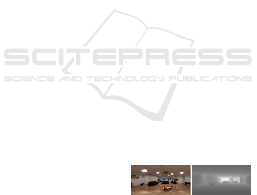
Figure 1: The radiance channel of the environment and the
depth channel used for reconstruct the light positions.
2 LIGHT-DEPTH MAP
A light-depth map contains both radiance and the
spatial displacement (i.e., depth) of the environment
light. The traditional approach for an environment
map is to take it as a set of infinite-distant or direc-
tional lights. In this new approach the map gives in-
formation about the geometry of the environment, so
we can consider it as a set of point lights instead of
directional lights.
209
René Zang A., Felinto D. and Velho L..
Rendering Synthetic Objects into Full Panoramic Scenes using Light-depth Maps.
DOI: 10.5220/0004216602090212
In Proceedings of the International Conference on Computer Graphics Theory and Applications and International Conference on Information
Visualization Theory and Applications (GRAPP-2013), pages 209-212
ISBN: 978-989-8565-46-4
Copyright
c
2013 SCITEPRESS (Science and Technology Publications, Lda.)
indent A pixel sample from the light-depth map is de-
noted by M(ω
i
,z
i
), where ω
i
is the direction of the
light sample in the map and the scalar value z
i
de-
notes the distance of the light sample from the light
space origin. The light sample position in light space
is given by the point z
i
ω
i
.
3 RENDERING USING
LIGHT-DEPTH MAPS
Our rendering system is based on the ray tracing algo-
rithm. For render synthetic elements into a real scene
photo-realistically, our system implements some ray
tracing tasks differently. We will discuss the aspects
that differ from the traditional approach to lead the in-
troduction of the rendering algorithm for augmented
scenes.
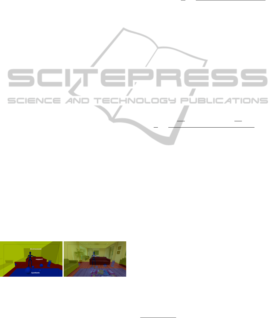
3.1 Scene Primitives
Our rendering system needs a special classification of
the scene primitives, figure 2, where each category
defines different light scattering contributions.
Synthetic Primitives: the objects that are new to the
scene. They don’t exist in the original environment.
Their light scattering calculation does not differ from
a traditional rendering algorithm, eq. (1).
Support Primitives: surfaces present in the original
environment that needs to receive shadows and re-
flections from the synthetic primitives. Their light
scattering calculation is not trivial, because it needs
to converge to the original lighting, eq. (3).
Environment Primitives: all the surfaces of the orig-
inal environment that need to be taken into account
for the reflections and shadows computations for the
other primitive types. They don’t require any light
scattering calculation, because their color is com-
puted directly from the light-depth map, eq. (2).
Figure 2: Primitives classification: synthetic (blue), support
(red) and environment (olive) primitives.
3.2 Surface Scattering
The computation of the direct lighting contribution,
L
o
(p,ω
o
), depends on the primitive type of p. Thus,
for each type of primitive, we have a particular way
to compute the contribution
• Synthetic Primitives: L
o
(p,ω
o
) is computed us-
ing the traditional Monte Carlo estimator
L
o
(p,ω
o
) =
1
N
N
∑
j=1
f (p,ω
o
,ω
j
)L
d
(p,ω
j
)|cosθ
j
|
pd f (ω
j
)
(1)
• Environment Primitives: direct lighting contribu-
tion is obtained directly from the light-depth map
as
L
o
(p,ω
o
) = M(ω
p
/|ω
p
|,|ω
p
|), (2)
where ω
p
= WT L(p).
1
• Support Primitives: Support surfaces need to be
rendered to include shadows and reflections from
the synthetic objects. The rendered value of a sup-
port point p that doesn’t have any contribution
from the synthetic objects must converge to the
radiance value stored in the light-depth map for
its position. Thus L
o
(p,ω
o
) is computed by the
estimator
1
N
N
∑
j=1
M(
ω
p
|ω
p
|
,|ω
p
|) · ES(p,n
p
) ·
D
¯
ω
j
|
¯
ω
j
|
,n
p
E
p(ω
j
)
, (3)
and ES(p, n
p
) denotes a special scale factor term,
used instead the BSDF term f (p, ω
o
,ω
j
), that rep-
resents the percentage of light contribution com-
ing from the map to the point p.
3.3 Shadows
For every ray that intersects with the scene at a point
p on a surface, the integrator takes a light sample ω
i
from the environment map to compute the light con-
tribution for p. Next, the renderer performs a visibil-
ity test to determine if the sampled light is visible or
not from the point p.
The integrator uses the light sample position in
real world and not only its direction to determine vis-
ibility. The visibility test is performed using the light
sample direction ω
i
and multiplying it by its depth
value z
i
to obtain the point z
i
· ω
i
in the light coordi-
nate system. The point z
i
· ω
i
is transformed to world
space (LTW) to obtain l
i
= LTW (z
i
· ω
i
). Thus the
visibility account is computed for the ray r(p,l
i
− p)
instead r(p, ω
i
) (see figure 3).
1
W T L(p) transform p from world space to light space.
GRAPP2013-InternationalConferenceonComputerGraphicsTheoryandApplications
210

Cam
p
Environment Map
Environment
primitive
support
primitive
synthetic
primitive
r(p, LTW(w
i
))
l
i
w
i
r(p, l
i
-p)
Figure 3: The shadows accounts.
3.4 Reflections
Given a point p on a surface, the integrator takes a
direction ω
i
by sampling the surface BRDF (Bidi-
rectional Reflectance Distribution Function) to add
reflection contributions to point p. In order to do
that, the renderer computes the intersection of the
ray r(p, ω
i
) with origin p and direction ω
i
with the
scene. If the intersection point q is over a synthetic or
a support surface its scattering contribution must be
added to the reflection account as it would normally.
Otherwise, if the intersection was with an environ-
ment mesh, q is transformed from world space to light
space (WTL) by computing q
L
= W T L(q). The con-
tribution given by the q
L
direction in the light-depth
map is then added to the reflection account (figure 4).
Cam
p
q
n
p
Environment Map
Environment
primitive
support
primitive
synthetic
primitive
w
i
r(p,w
i
)
O
E
q
L
Figure 4: Reflection account.
4 AUGMENTED PATH TRACING
We solve the light transport equation by constructing
the path incrementally, starting from the vertex at the
camera p
0
.
For each vertex p
k
with k = 1,· · · ,i − 1 we com-
pute the radiance scattering at point p
k
along the
p
k−1
− p
k
direction. The scattering computation for
p
k
on a synthetic, support or environment surface is
performed using respectively the equations (1), (3)
and (2).
A path ¯p
i
= (p
0
,··· , p
i
) can be classified accord-
ing the nature of its vertices as
• Real Path: the vertices p
k
, k = 1,··· , i − 1 are on
support surfaces.
• Synthetic Path: the vertices p
k
, k = 1,··· ,i − 1
are on synthetic objects surfaces.
• Mixed Path: some vertices are on synthetic ob-
jects and other on support surfaces.
There is no need to calculate any of the real path
for the light. They are already present in the original
photography. However, since part of the local scene
was modeled (and potentially modified), we need to
re-render it for these elements. The calculated radi-
ance needs to match the captured value from the envi-
ronment. We do this by aggregating all the real path
radiance in a vertex p
1
as direct illumination, discard-
ing the need of considering the neighbor vertices light
contribution.
The synthetic and mixed light paths are calculated
in a similar way, taking the individual path vertex light
contributions for every vertex of the light path. The
difference between them is in the Monte Carlo esti-
mate applied in each case. In the figure (5) you can
see the different light path types and the calculation
that happens on the corresponding path vertices.
p
0
p
1
p
2
Support surfaces
Synthetic objects
p
0
p
1
p
2
p
0
p
1
p
2
p
3
p
4
p
3
Real path
Synthetic path
Mix path
Direct lighting contribution
p
4
p
5
Figure 5: Path type classification. The yellow cones shows
which vertices contributes for direct lighting account.
5 RESULTS AND CONCLUSIONS
The rendering performance of our approach is equiva-
lent to the rendering of a normal scene with the same
mesh complexity using a physically based light ren-
dering algorithm. There was no visible lost in that
regard. Part of the merit of this, is that this is an
one-pass solution. There is no need for multiple com-
position passes. The rendering solution converges to
the final results without ”adjustments” loops been re-
quired like Debevec’s approach (Debevec, 1998).
The mirror ball reflection calculation can be seen
in more details in the figure 6. This is a compari-
son between the traditional directional map method
and our light-depth solution. The spheres and the
carpet are synthetic and render the same with both
methods. The presence of the original environment
RenderingSyntheticObjectsintoFullPanoramicScenesusingLight-depthMaps
211
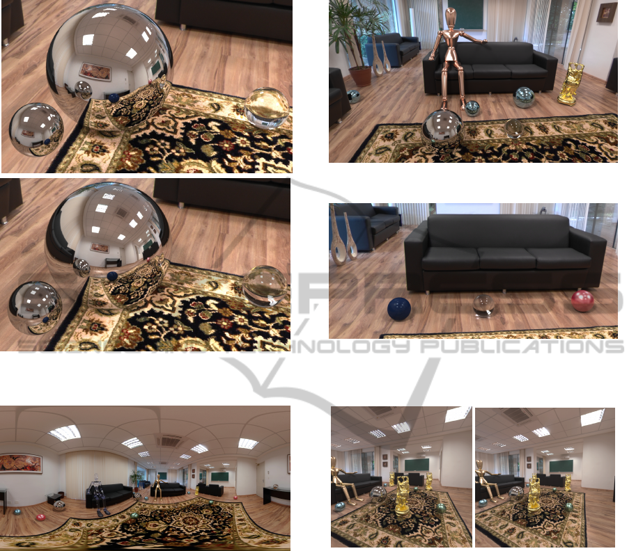
Figure 6: Comparison between reflections given by direc-
tional map (upper) and light-depth map (lower) approaches.
Figure 7: Rendering of a full panoramic scene with syn-
thetic objects. All the balls and the dolls in the scene are
synthetics. The carpet on the floor was synthesized to cover
a table that is in the original environment capture.
meshes makes the reflection to be a continuous be-
tween the synthetic (e.g., carpet) and the environment
(e.g., wood floor).
The proper calibration of the scene and the cor-
rect shadows helps the natural feeling of belonging
for the synthetic elements in the scene. In figures 8
and 9 you can see a non panoramic frustum of figure
7 to showcase the correct perspective when seen in a
conventional display.
Finally, we explored camera traveling for a few of
our shots. In the figure 10 you can see part of the
scene rendered from two different camera positions.
The result is satisfactory as long as the support envi-
ronment match is properly modeled. For slight cam-
era shifts this is not even a problem.
Figure 8: Limited frustum view of the figure 7.
Figure 9: Shadows computed using the light-depth map.
The orientation of the shadows varies respecting the posi-
tion of the balls in the scene.
Figure 10: Camera traveling effect. Two points of views us-
ing camera position displaced from the environment origin.
Among the possible improvements, we are inter-
ested on studying techniques to recover the light posi-
tions for assembling the light-depth environment map
and semi-automatic environment mesh construction
for the cases where we can capture a point cloud of
the environment geometry.
REFERENCES
Debevec, P. E. (1998). Rendering synthetic objects into real
scenes: Bridging traditional and image-based graph-
ics with global illumination and high dynamic range
photography. pp. 189-198. SIGGRAPH.
Felinto, D. Q., Zang, A. R., and Velho, L. (2012). Produc-
tion framework for full panoramic scenes with photo-
realistic augmented reality. In XXXVIII Latin Ameri-
can Conference of Informatics (CLEI), Medellin.
GRAPP2013-InternationalConferenceonComputerGraphicsTheoryandApplications
212
