On using Additional Unlabeled Data for Improving
Dissimilarity-Based Classifications
∗
Sang-Woon Kim
Dept. of Computer Engineering, Myongji University, Yongin 449-728, Republic of Korea
Keywords:
Dissimilarity-Based Classification (DBC), One-Shot Similarity Metric (OSS), Semi-Supervised Learning
(SSL).
Abstract:
This paper reports an experimental result obtained with additionally using unlabeled data together with labeled
ones to improve the classification accuracy of dissimilarity-based methods, namely, dissimilarity-based clas-
sifications (DBC) (Pe¸kalska, E. and Duin, R. P .W., 2005). In DBC, classifiers among classes are not based on
the feature measurements of individual objects, but rather on a suitable dissimilarity measure among the ob-
jects. In image classification tasks, on the other hand, one of the intractable problems is the lack of information
caused by the insufficient number of data. To address this problem in DBC, in this paper we study a new way
of measuring the dissimilarity distance between two object images by using the well-known one-shot similar-
ity metric (OSS) (Wolf, L. et al., 2009). In DBC using OSS, the dissimilarity distance is measured based on
unlabeled (background) data that do not belong to the classes being learned, and consequently, do not require
labeling. From this point of view, the classification is done in a semi-supervised learning (SSL) framework.
Our experimental results, obtained with well-known benchmarks, demonstrate that when the cardinalities of
the unlabeled data set and the prototype set have been appropriately chosen using additional unlabeled data
for the OSS metric in SSL, DBC can be improved in terms of classification accuracies.
1 INTRODUCTION
In dissimilarity-based classifications (DBC), design-
ing a classifier is not based on the feature measure-
ments of individual objects, but rather on a suitable
dissimilarity measure among the individual objects
(Pe¸kalska, E. and Duin, R. P .W., 2005). The advan-
tage of this strategy is that it can avoid the problems
associated with feature spaces, such as the curse of
dimensionality and the issue of estimating a number
of parameters on data distributions (Kim, S. -W. and
Oommen, B. J., 2007). Another characteristic of the
dissimilarity approach is that it offers a different way
to include expert knowledge on the objects in classi-
fying them (Duin, R. P .W., 2011). One of the ques-
tions we encountered when designing DBC is: How
can the (dis)similarities between object examples be
efficiently measured? To explore this question, vari-
ous strategies have been proposed in the literature, in-
cluding (Bicegoa, M. et al., 2004), (Pe¸kalska, E. and
Duin, R. P .W., 2005), (Pe¸kalska, E. and Duin, R. P
∗
This work was supported by the National Research
Foundation of Korea funded by the Korean Government
(NRF-2012R1A1A2041661).
.W., 2008), (Orozco-Alzate, M. et al., 2009), (Duin,
R. P .W., 2011), and (Mill
´
an-Giraldo, M. et al., 2012).
In these strategies, investigations have focused specif-
ically on generalizing the dissimilarity representation
by using various methods, such as feature lines and
feature planes (Orozco-Alzate, M. et al., 2009) and
hidden Markov models (Bicegoa, M. et al., 2004).
On the other hand, when designing a DBC with a
measuring system, we sometimes suffer from the dif-
ficulty of collecting sufficient (labeled) training data
for each class. Labeled instances, for example, are
often difficult, expensive, or time-consuming to ob-
tain, as they require the services of an experienced ex-
pert. Meanwhile, unlabeled data, defined as the sam-
ples that do not belong to the classes being learned,
may be relatively easy to collect, but the use of this
type of data is limited. To address this problem,
in a learning framework of semi-supervised learning
(SSL) (Chapelle, O. et al., 2006), a large amount of
unlabeled data, together with labeled data, can be uti-
lized to build better classifiers. Because SSL requires
less human effort and results in higher accuracy, it is
of great interest in practice. However, it is also well
known that the utilization of unlabeled data is not al-
132
Kim S. (2013).
On using Additional Unlabeled Data for Improving Dissimilarity-Based Classifications.
In Proceedings of the 2nd International Conference on Pattern Recognition Applications and Methods, pages 132-137
DOI: 10.5220/0004218901320137
Copyright
c
 SciTePress

ways helpful for SSL. Specifically, it is not guaran-
teed that adding unlabeled data to the training data
leads to a situation in which we can improve the per-
formance (Ben-David, S. et al., 2008). Several strate-
gies have been investigated to address this, including
self-training (McClosky, D. et al., 2008), co-training
(Blum, A. and Mitchell, T., 1998), SemiBoost (Mal-
lapragada, P. K. et al., 2009), etc.
Recently, one-shot similarity (OSS) (Wolf, L.
et al., 2009) was proposed to exploit both labeled and
unlabeled (background) data when learning a classifi-
cation model. In OSS, when given two vectors, x
i
and
x
j
, and an additionally available (unlabeled) data set,
A, a measure of the (dis)similarity between x
i
and x
j
is computed as follows: First, a discriminative model
is learned with x
i
as a single positive example and A
as a set of negative examples. This model is then used
to classify x
j
, and to obtain a confidence score. Next,
a second such score is obtained by repeating the same
process with the roles of x
i
and x
j
switched. Finally,
the (dis)similarity of the two vectors can be obtained
by averaging the above two scores.
In DBC, on the other hand, when a limited num-
ber of objects are available, it is difficult to achieve the
desired classification performance. To overcome this
limitation, in this paper we study a way of exploit-
ing additionally available unlabeled data when mea-
suring the dissimilarity distance with the OSS metric.
As in SSL, we use the easily collected unlabeled data
as the background data set, A, with which we can en-
rich the representational capability of the dissimilarity
measures. The main contribution of this paper is to
demonstrate that the classification accuracy of DBC
can be improved by employing the OSS metric based
on additional unlabeled data. More specifically, ex-
periments on an artificial and real-life data sets have
been carried out to demonstrate better performance
than selected baseline approaches.
The remainder of the paper is organized as fol-
lows: In Section 2, after providing a brief introduction
to DBC and OSS, we present an explanation for the
use of OSS in DBC and a modified DBC algorithm. In
Section 3, we present the experimental setup and the
results obtained with the experimental data. Finally,
in Section 4, we present our concluding remarks as
well as some feature works that deserve further study.
2 RELATED WORK
2.1 Dissimilarity Representation
A dissimilarity representation of a set of objects, T =
{
x
i
}
n
i=1
∈ R
d
(d-dimensional samples), is based on
pair-wise comparisons, and is expressed, for exam-
ple, as an n × m dissimilarity matrix, D
T,P
[·, ·], where
P =
{
p
j
}
m
j=1
∈ R
d
, a prototype set, is extracted from
T . The subscripts of D represent the set of elements,
on which the dissimilarities are evaluated. Thus, each
entry, D
T,P
[i, j], corresponds to the dissimilarity be-
tween the pairs of objects, ⟨x
i
, p
j
⟩, where x
i
∈ T and
p
j
∈ P. Consequently, when given a distance measure
between two objects, d(·, ·), an object, x
i
, (1 ≤ i ≤ n),
is represented as a new vector, δ(x
i
, P), as follows:
δ(x
i
, P) = [d(x
i
, p
1
), d(x
i
, p
2
), ··· , d(x
i
, p
m
)]. (1)
Here, the generated dissimilarity matrix, D
T,P
[·, ·],
defines vectors in a dissimilarity space, on which
the d-dimensional object, x, given in the input fea-
ture space, is represented as an m-dimensional vec-
tor, δ(x, P) or shortly δ(x). On the basis of what we
have just explained briefly, a conventional algorithm
for DBC is summarized as follows:
1. Select the prototype subset, P, from the training
set, T , by using one of the prototype selection meth-
ods described in the related literature.
2. Using Eq. (1), compute the dissimilarity ma-
trix, D
T,P
[·, ·], in which each dissimilarity is computed
on the basis of the given distance measure d(·, ·).
3. For a testing sample, z, compute a dissimilar-
ity feature vector, δ(z), by using the same prototype
subset and the distance measure used in Step 2.
4. Achieve the classification by invoking a classi-
fier built in the dissimilarity space and operating it on
the dissimilarity vector δ(z).
2.2 One-shot Similarity
Assume that we have two vectors, x
i
and x
j
, and an
additionally available (unlabeled) data set, A. To mea-
sure OSS, we first generate a hyperplane that sepa-
rates x
i
and A (and also x
j
and A). Then, we count
the distance from x
j
(and also x
i
) to the hyperplane
decision surface. For a 2-class classification problem,
for example, we begin with a simple case of design-
ing a linear classifier described by g(x) = w
T
x + w
0
.
To make it clear, we focus again on the binary LDA
(Fisher’s linear discriminant analysis) (Duda, R. O.
et al., 2001). Then, after deriving a projection ma-
trix, w, by maximizing the Rayleigh quotient, we can
classify an unknown vector, z, to class-1 (or class-2)
if g(z) > 0 (or g(z) < 0).
Using the above LDA-based OSS, the dissimilar-
ity distance between the pairs of x
i
and x
j
can be com-
puted as follows (Wolf, L. et al., 2011):
1. By assuming that the class-1 contains a single
vector x
i
and the class-2 corresponds to the set of A,
OnusingAdditionalUnlabeledDataforImprovingDissimilarity-BasedClassifications
133

we compute the absolute distance of x
i
to the hyper-
plane that separates x
j
and A,
|g(x
i
)|
∥w∥
, where | · | (and
∥ · ∥) denotes the absolute value of a scaler (and the
Euclidean norm of a vector), as follows:
γ(x
i
, x
j
, A) =
|(x
j
− µ
A
)
T
S
−1
W
(x
i
−
x
j
+µ
A
2
)|
∥S
−1
W
(x
j
− µ
A
)∥
, (2)
where µ
A
(and S
−1
W
) denotes the mean of all vectors
(and the pseudo-inverse of the within-class covariance
matrix) of A. Also, the bias term is computed using w
and the mean of x
j
and µ
A
, as: w
0
= −w
T
x
j
+µ
A
2
.
2. By repeating the same process with the roles of
x
i
and x
j
switched, we compute the distance of x
j
to
the hyperplane that separates x
i
and A as follows:
γ(x
j
, x
i
, A) =
|(x
i
− µ
A
)
T
S
−1
W
(x
j
−
x
i
+µ
A
2
)|
∥S
−1
W
(x
i
− µ
A
)∥
. (3)
3. Finally, by averaging these two distances, we
can compute the dissimilarity of Eq. (1) as follows:
d
OSS
(x
i
, x
j
) =
1
2
(γ(x
i
, x
j
, A) + γ(x
j
, x
i
, A)), (4)
where x
j
plays as a p
j
, (1 ≤ j ≤ m).
2.3 The Use of OSS for DBC
When given an unlabeled data set, A ∈ R
d
, l = |A|
(where |·| denotes the cardinality of a set), in addition
to the existing prototype set, P, m = |P|, the cardinal-
ity of the representation set, P
′
(= P∪A ∈ R
d
), is m+l
when the entire set of the training data is selected as
the prototypes. Thus, each entry of the dissimilarity
matrix, D
T,P
′
[i, j], (1 ≤ i ≤ n; 1 ≤ j ≤ m + l), is repre-
sented as an augmented vector, δ(x
i
, P
′
), as follows:
δ(x
i
, P
′
) = [d(x
i
, p
1
), d(x
i
, p
2
), ··· , d(x
i
, p
m+l
)], (5)
where p
j
∈ P
′
and m + l = |P
′
|.
In DBC, another way of utilizing A is to measure
the dissimilarity in OSS metric by employing A as the
background data. When measuring the OSS together
with A, each entry of D
T,P
[i, j], (1 ≤ i ≤ n; 1 ≤ j ≤ m),
is computed as follows:
δ
OSS
(x
i
, P) = [d
OSS
(x
i
, p
1
), ··· , d
OSS
(x
i
, p
m
)], (6)
where p
j
∈ P and m = |P|.
On the basis of what we explained briefly, an al-
gorithm for SSL-type DBC is summarized as follows:
1. Obtain labeled training set T , prototype subset
P, and unlabeled set A as input data sets.
2. Using Eq. (5) or (6), rather than Eq. (1),
compute D
T,P
[·, ·], in which each dissimilarity is com-
puted on the basis of a distance metric.
3. This step is the same as Step 3 in DBC.
Table 1: Characteristics of the experimental data sets. Here,
the dimensionality of the data set marked with a
†
symbol
is reduced into 10% value using a PCA.
Data Datasets # of # of # of
types names features classes objects
Auto mpg 6 2 392
Dermatology 34 6 366
Diabetes 8 2 768
UCI Heart 13 2 297
Laryngeal1 16 2 213
Liver 6 2 345
Nist38 1024 2 1000
Sonar 60 2 208
Yeast 8 10 1484
BCI 117 2 400
COIL 241 6 1500
SSL COIL2 241 2 1500
USPS 241 2 1500
Text
†
11960 2 1500
4. This step is the same as Step 4 in DBC.
From a comparison of the algorithms of DBC and
SSL-type DBC given in Sections 2.1 and 2.3, it can be
seen that the required CPU-time for the latter is more
sensitive to the dimensionality and the cardinality of
T , P, and A than that for the former.
3 EXPERIMENTAL RESULTS
3.1 Experimental Setup
The proposed method has been tested and compared
with the conventional ones. This was done by per-
forming experiments on an artificial data, namely,
the Difficult (a normally distributed d-dimensional
2-class) data (Duin, R. P .W. et al., 2004)
2
and
other multivariate data sets cited from the UCI ma-
chine learning repository (Frank, A. and Asuncion,
A., 2010)
3
and SSL-type benchmarks (Chapelle, O.
et al., 2006)
4
. Characteristics of the UCI and SSL-
type data sets are summarized in Table 1.
The experiment focuses on a few simple binary
and multi-class classification problems, where all data
sets are initially split into three subsets: labeled train-
ing data, L, labeled test (evaluation) data, E, and un-
labeled data, U . The training and test procedures are
then repeated ten times and the results obtained are
averaged.
In this experiment, classifications are carried out
in four ways, which are named F
input
, D
excl ude
,
2
http://prtools.org/
3
http://www.ics.uci.edu/∼mlearn/MLRepository.html
4
http://www.kyb.tuebingen.mpg.de/ssl-book/
ICPRAM2013-InternationalConferenceonPatternRecognitionApplicationsandMethods
134

D
include
, and D
OSS
. In F
input
, classification is carried
out in the original input-feature space as the tradi-
tional one does. In the other schemes, however, clas-
sifications are performed in three dissimilarity repre-
sentations differently constructed as follows: First, in
D
excl ude
approach, the entire L (or its subset) serves
as a prototype set P, and the dissimilarity between the
pairwise objects, δ(·, P), is measured with Eq. (1),
in which d(·, ·) is the Euclidean distance (l
2
metric).
Here, U is precluded. Second, in D
include
, the pro-
totype set, P, is randomly selected from L ∪ U and
the dissimilarity, δ(·, P), is measured with Eq. (5),
in which d(·, ·) is also l
2
metric. Finally, in D
OSS
,
L works as the prototype set P, and the dissimilar-
ity, δ
OSS
(·, P), is measured with Eq. (6), in which
d
OSS
(
·
,
·
)
is the averaged OSS confidence,
¯
γ
(
·
,
·
,
·
)
, uti-
lizing U as a A. Here, to select prototypes from L
or L ∪U, the Random selection is utilized in the ex-
periment. However, other various methods described
in the literature (Pe¸kalska, E. and Duin, R. P .W.,
2005), (Kim, S. -W. and Oommen, B. J., 2007), such
as RandomC, KCentres, ModeSeek, LinProg, FeatSel,
KCentres-LP, EdiCon, etc, can also be considered.
Finally, to evaluate the classification accuracies of
all the four approaches, a classifier based on the k-
nearest neighbor rule is employed to classify the eval-
uation test data, E (or the corresponding dissimilarity
representations), and will be denoted as knnc (where
k = 1) in subsequent sections.
3.2 Experiment # 1 (Difficult Data)
First, the experimental results obtained with the three
classifiers trained in the four approaches for an arti-
ficial data set, the Difficult data set (Duin, R. P .W.
et al., 2004), were probed into. We first generated a
5-dimensional 2-class Difficult data set of the positive
and negative samples of [300, 300], and divided them
into L, E, and U subsets at a ratio of 20% : 10% : 70%.
Then, we performed the experiment as mentioned
previously.
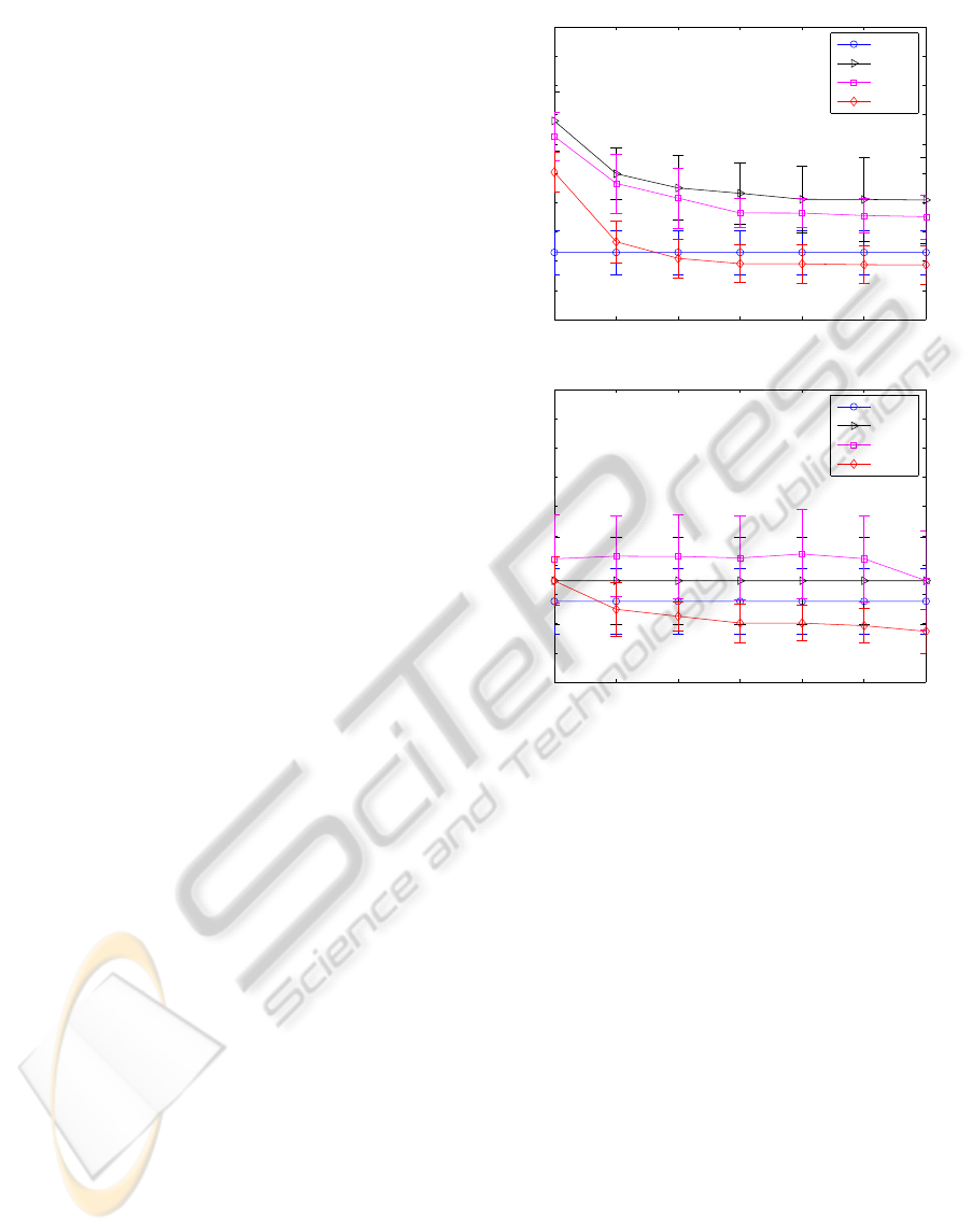
Fig. 1 (a) shows a comparison of the error rates
obtained with knnc trained in the four approaches for
seven different cardinalities of P of Difficult data, un-
der the condition A = U. Also, Fig. 1 (b) shows a
comparison of the error rates obtained with the same
classifier, but designed with different cardinalities of
A of Difficult, having P = L. Here, the x and y axes
represent the seven different cardinalities of P (and A)
and the averaged error rates, respectively.
The observations obtained from the two pictures
shown in Fig. 1 (a) and (b) are the followings: First,
in Fig. 1 (a), it should be pointed out that the esti-
mated error rates obtained with the D
excl ude
, D
include
,
2 5 10 20 30 50 120
0
0.05
0.1
0.15
0.2
0.25
0.3
0.35
0.4
0.45
0.5
Difficult−knnc
The cardinality of prototype set (P)
Error rates
F
input
D
exclude
D
include
D
OSS
2 5 10 20 30 50 420
0
0.05
0.1
0.15
0.2
0.25
0.3
0.35
0.4
0.45
0.5
Difficult−knnc
The cardinality of unlabeled (background) set (A)
Error rates
F
input
D
exclude
D
include
D
OSS
Figure 1: Error rates obtained with knnc trained in the four
approaches for Difficult data: (a) top and (b) bottom; (a) and
(b) are obtained with different cardinalities of the prototype
set, P, and the unlabeled data set, A, respectively.
and D
OSS
approaches, marked with the ◃, , and ⋄
symbols, decrease uniformly as the cardinality of P
increases, i.e., the three graphs have the same shape
in general, maintaining a consistent difference from
each other. This comparison demonstrates that the
classification accuracy of D
OSS
, marked with the ⋄
symbol, is always the lowest among the four rates
when having an appropriate number of prototypes.
Next, in Fig. 1 (b), the two error rates obtained
with D
excl ude
and D
include
are almost the same for dif-
ferent numbers of unlabeled samples, from which we
can see that the addition of an available unlabeled data
set, U , to the existing prototype set, i.e., P = L ∪U or
its randomly selected subsets, did not succeed in en-
hancing the classification performance.
Finally, in Fig. 1 (b), it should be mentioned that,
in evaluation of the error rates, the cardinality of the
prototype set is more sensitive than that of the unla-
beled background set; the curves of the latter are more
flat than those of the former.
From these observations, it can be mentioned that
OnusingAdditionalUnlabeledDataforImprovingDissimilarity-BasedClassifications
135

the accuracy of certain kinds of DBC classifiers, such
as knnc, can be improved by using the available un-
labeled data in a SSL fashion through measuring the
dissimilarity with a OSS metric. This characteristic
can be observed again in subsequent experiments.
3.3 Experiment # 2 (UCI / SSL Data)
Second, to further investigate the characteristics of the
proposed method, and, especially, to find out which
kinds of significant data sets are more suitable for
the scheme, we repeated the experiment with a few
of UCI and SSL-type benchmark data sets. After di-
viding each data set into the L, E, and U subsets at a
ratio of 40% : 30% : 30%, we performed the training
and evaluation procedures 30 times and computed the
error rates by averaging the results obtained.
Table 2 shows a numerical comparison of
the mean error rates (
±
standard deviations) ob-
tained with the classifier, knnc, trained in a tradi-
tional feature-based and four dissimilarity-based ap-
proaches. Here, the results shown in the fifth and the
sixth columns, i.e., those of D
includeP
and D
includeW
,
are obtained with two specific cases of D
include
. In the
latter case, the prototype set is the whole set of labeled
samples and unlabeled ones, i.e., P = L ∪ U, while,
in the former case, it is the (randomly chosen) par-
tial subset of the cardinality of |L|. Besides, in both
D
excl ude
and D
OSS
, the entire set of L is served as a P,
while, in D
OSS
, U is utilized as a A. Also, in order to
facilitate the comparison in the tables, the lowest er-
ror rate in each data set is bold-faced. Especially, the
values highlighted with a
∗
marker are the lowest one
among the four error rates of the DBC approaches.
Table 2 presents the error rates obtained with knnc
designed in the five approaches for the data sets,
showing the similar characteristics as the ones we
obtained in the figures (see the bold-faced and/or
∗
marked numbers). In the table, we observed that al-
most all of the lowest error rates (
∗
marked) were
achieved with D
OSS
except for Auto mpg.
From this consideration, a question arises: Why
does D
OSS
not work in certain applications? The the-
oretical explanation for this remains unchallenged.
In addition, to simplify the classification task for
the experiment and because of the limit on the num-
ber of pages, only a classifier of the k-nearest neigh-
bor rule was experimented and analyzed. However,
other classifiers, including the AdaBoost algorithm,
support vector machines, and neural networks, can
also be considered.
Also, in the above two experiments # 1 and # 2, it
was observed that using U can lead to increasing the
classification accuracy of DBC. Although the class-
labels of the U was not used in the training phase,
it had been selected from a given training data set.
Thus, the characteristics of U are the same as those
of the training data set. From this point of view, the
following question is an interesting issue to investi-
gate: Is the classification accuracy of D
OSS
superior
or inferior to that of the conventional scheme when
U is collected from a different data set? The exper-
imental results on these issues will be appeared in a
subsequent journal paper.
In review, it is not easy to decide which kinds of
significant methods are more suitable for DBC to use
unlabeled data in a SSL fashion. However, by com-
paring the numbers of the highlighted values among
the DBC approaches, the reader should observe that
the classification accuracies of certain kinds of classi-
fiers designed with D
OSS
, representing the use of OSS
for DBC, are marginally better than those of the clas-
sifiers designed in D
exclude
, D
includeP
, and D
includeW
.
So, the classifier of D
OSS
, albeit not always, seems to
be more helpful for certain kinds of data sets than the
Euclidean distance does.
4 CONCLUSIONS
In our efforts to improve the classification perfor-
mance of DBC in a SSL fashion, we used the well-
known OSS measuring scheme based on the back-
ground information of available extra (unlabeled)
data. To achieve this improvement, we first com-
puted the confidence levels of the training data with
the OSS metric. We then constructed the dissimilarity
matrices, where the dissimilarity was measured with
the averaged confidence levels. This measuring tech-
nique using unlabeled data was employed to solve the
problems caused by the insufficient number of labeled
data. The proposed method was tested on an artificial
data and the UCI / SSL-type data sets, and the results
obtained were compared with those of a feature-based
classification and three dissimilarity-based ones.
Our experimental results demonstrate that the
classification accuracy of DBC, albeit not always, is
improved when the cardinalities of the prototype sub-
set P and the unlabeled background set A have been
appropriately chosen. Also, the results show that
the accuracy is superior to that of the conventional
schemes when A is collected from data samples that
are different in nature. Although we have shown that
DBC can be improved by employing the OSS metric,
many tasks remain open. One of them is to further
improve the classification efficiency by selecting an
optimal, or nearly optimal, cardinality of P (and A)
and utilizing various distance learning techniques in
ICPRAM2013-InternationalConferenceonPatternRecognitionApplicationsandMethods
136

Table 2: A numerical comparison of the mean error (± std) rates obtained with knnc implemented in the five approaches
for the UCI and SSL-type data sets. In order to facilitate the comparison, for each row, the lowest error rate is bold-faced.
Especially, the values highlighted with a
∗
marker are the lowest one among the four error rates of the DBC approaches.
Data Dataset Input feature-based Dissimilarity-based classification (DBC)
types names classification (F
input
) D
exclude
D
includeP
D
includeW
D
OSS
Auto mpg 15.00 ± 2.49 15.00 ± 2.71 15.20 ± 2.68
∗
14.94 ± 2.62 14.97 ± 3.16
Dermatology 16.35 ± 3.78 32.86 ± 4.37 34.00 ± 3.89 32.79 ± 4.11
∗
14.44 ± 3.59
Diabetes 28.60 ± 2.62 29.80 ± 2.40 29.99 ± 2.41 29.51 ± 2.42
∗
27.22 ± 1.85
UCI Heart 36.78 ± 4.59 40.45 ± 4.27 40.42 ± 4.16 40.68 ± 4.27
∗
35.11 ± 3.84
Laryngeal1 25.22 ± 5.38 32.90 ± 5.42 33.49 ± 5.55 32.90 ± 6.12
∗
24.62 ± 5.26
Liver 34.51 ± 5.11 40.03 ± 4.36 40.26 ± 4.16 40.39 ± 4.32
∗
36.50 ± 5.37
Nist38 2.90 ± 0.75 2.98 ± 0.90 4.44 ± 1.31 3.06 ± 0.92
∗
2.66 ± 1.03
Sonar 24.44 ± 6.10 28.28 ± 5.76 29.89 ± 4.75 28.94 ± 7.04
∗
24.72 ± 6.74
Yeast 43.55 ± 2.23 46.04 ± 2.11 46.03 ± 2.03 46.17 ± 2.38
∗
43.45 ± 2.33
BCI 46.06 ± 4.97 46.89 ± 4.58 47.00 ± 4.98 47.78 ± 4.18
∗
44.72 ± 4.99
COIL 5.72 ± 1.35 6.44 ± 1.07 6.58 ± 1.17 6.56 ± 1.11
∗
4.93 ± 1.08
SSL COIL2 0.81 ± 0.51 1.90 ± 0.83 2.01 ± 0.79 1.92 ± 0.79
∗
0.60 ± 0.43
USPS 3.73 ± 0.94 4.81 ± 1.01 4.79 ± 0.95 4.81 ± 0.87
∗
3.52 ± 0.81
Text 23.67 ± 1.86 24.22 ± 1.98 26.44 ± 2.36 24.36 ± 2.10
∗
22.35 ± 2.06
the OSS scheme. Also, it is not yet clear which kinds
of significant data sets (and classifiers) are more suit-
able for the use of OSS for DBC.
Finally, the proposed method lacks of details to
support its technical soundness, and the experiments
performed are very limited. Therefore, the problem of
theoretically investigating the measuring method de-
veloped for DBC remains to be challenged.
REFERENCES
Ben-David, S., Lu, T., and Pal, D. (2008). Does unlabeled
data provably help? Worst-case analysis of the sample
complexity of semi-supervised learning. In Proc. of
the 21st Annual Conf. on Learning Theory (COLT08),
pages 33–44, Helsinki, Finland.
Bicegoa, M., Murinoa, V., and Figueiredob, M. A. T.
(2004). Similarity based classification of sequences
using hidden markov models. Pattern Recognition,
37:2281–2291.
Blum, A. and Mitchell, T. (1998). Combining labeled
and unlabeled data with co-training. In Proc. of the
11th Annual Conf. on Computational Learning The-
ory (COLT 98), pages 92–100, Madison, WI.
Chapelle, O., Sch ¨olkopf, B., and Zien, A. (2006). Semi-
Supervised Learning. The MIT Press, MA.
Duda, R. O., Hart, P. E., and Stork, D. G. (2001). Pattern
Classification Second Edition. John Wiley & Sons.
Duin, R. P .W. (2011). Non-euclidean problems in pattern
recognition related to human expert knowledge. In
Proc. of ICEIS2010. Springer-Verlag.
Duin, R. P .W., Juszczak, P., de Ridder, D., Pacl
´
ık, P.,
Pe¸kalska, E., and Tax, D. M. J. (2004). PRTools 4:
A Matlab Toolbox for Pattern Recognition. Delft Uni-
versity of Technology, Delft, The Netherlands.
Frank, A. and Asuncion, A. (2010). UCI Machine Learning
Repository. University of California, School of Infor-
mation and Computer Science, Irvine, CA.
Kim, S. -W. and Oommen, B. J. (2007). On using pro-
totype reduction schemes to optimize dissimilarity-
based classification. Pattern Recognition, 40:2946–
2957.
Mallapragada, P. K., Jin, R., Jain, A. K., and Liu, Y.
(2009). Semiboost: Boosting for semi-supervised
learning. IEEE Trans. Pattern Anal. and Machine In-
tell., 31(11):2000–2014.
McClosky, D., Charniak, E., and Johnson, M. (2008). When
is self-training effective for parsing? In Proc. of the
22nd Int’l Conf. on Computational Linguistics (Coling
2008), pages 561–568, Manchester, UK.
Mill
´
an-Giraldo, M., Garc
´
ıa, V., and S
´
anchez, J. S. (2012).
Prototype selection in imbalanced data for dissimilar-
ity representation - A preliminary study. In Proc. of
the 1st Int’l Conf. on Pattern Recognition Applications
and Methods (ICPRAM 2012), pages 242–246.
Orozco-Alzate, M., Duin, R. P .W., and Castellanos-
Dominguez, G. (2009). A generalization of dissim-
ilarity representations using feature lines and feature
planes. Pattern Recognition Letters, 30:242–254.
Pe¸kalska, E. and Duin, R. P .W. (2005). The Dissimilarity
Representation for Pattern Recognition: Foundations
and Applications. World Scientific, Singapore.
Pe¸kalska, E. and Duin, R. P .W. (2008). Beyond traditional
kernels: Classification in two dissimilarity-based rep-
resentation spaces. IEEE Trans. Sys., Man, and Cy-
bern.(C), 38(6):727–744.
Wolf, L., Hassner, T., and Taigman, Y. (2009). The One-
Shot Similarity Kernel. In T. Matsuyama, C. Cipolla,
et al., editor, Proc. IEEE Intl Conf. Computer Vision,
pages 897–902. IEEE Computer Society Press.
Wolf, L., Hassner, T., and Taigman, Y. (2011). Ef-
fective unconstrained face recognition by combining
multiple descriptors and learned background statis-
tics. IEEE Trans. Pattern Anal. and Machine Intell.,
33(10):1978–1990.
OnusingAdditionalUnlabeledDataforImprovingDissimilarity-BasedClassifications
137