
The Pareto Frontier for Vehicle Fleet Purchases
Cost versus Sustainability
Daniel Reich, Sandra L. Winkler and Erica Klampfl
Ford Research & Advanced Engineering, Dearborn, Michigan 48124, U.S.A.
Keywords:
Integer Programming, Sustainability, Automotive.
Abstract:
Vehicle fleets for large corporations can have thousands of vehicles that are replaced between every few months
and every few years. With the emergence of hybrid, plug-in hybrid, and other new vehicle technologies,
combined with an increasing focus on sustainability, planning fleet purchases has and continues to become
a significantly more complicated undertaking. This paper introduces Ford’s Fleet Purchase Planner system
designed to present fleet customers with optimal purchase strategies that incorporate their companies’ cost
and sustainability considerations.
1 INTRODUCTION
Ford’s Fleet Purchase Planner (patent pending) is an
analytical system, using mathematical optimization
methodology, designed to help fleet customers better
understand purchase options. It provides customized
purchase recommendations that satisfy corporate en-
vironmental goals, reduce costs, and analyze trade-
offs between company goals.
Sustainability and environmental impact are ar-
eas of growing importance to many of Ford’s fleet
customers. For example, SimplexGrinnell ordered
200 Fusion Hybrids in 2010 to support a Tyco
company-wide environmental program, known as
”Vital World,” to reduce greenhouse gas emissions,
waste and water consumption by 25 percent over the
next five years (Ford Motor Company, 2010b). Kraft
also has goals with its sales fleet program to reduce
fuel use and CO
2
emissions and purchased 4 cylinder
Fusions in 2010 to help accomplish this (Ford Motor
Company, 2010a).
In recent years, several new green vehicle tech-
nologies have emerged, e.g., battery electric vehi-
cles (BEVs), hybrid electric vehicles (HEVs), plug-
in HEVs (PHEVs), and turbocharged direct injected
gasoline engines (e.g., Ford’s EcoBoost
R
). These
technologies provide increasing opportunities for cus-
tomers to reduce emissions and operating costs, but
they also increase the number of purchase options
available, making planning a more complicated en-
deavor.
For example, what is the trade-off cost for pur-
chasing a Focus versus a Focus Electric (BEV)? Can
a company recover the additional cost incurred in
purchasing the BEV through fuel savings over time?
Does a BEV have the same emissions if driven in Cal-
ifornia as it does in Michigan, Texas or Florida? Deci-
sions become even more complex as customers need
to choose which vehicles in their existing fleet to re-
place, which vehicles they should replace them with
(e.g. Focus, Focus Electric, Fusion, Fiesta), and how
these choices enable them to meet their cost and sus-
tainability targets.
This paper presents details on our Fleet Purchase
Planner (FPP) and is organized as follows. In Section
2, we provide background information on measuring
a vehicle’s carbon footprint. Section 3 introduces our
algorithm and integer programming models used to
generate optimal purchase recommendations. In Sec-
tion 4, we demonstrate our software application on an
example fleet. Section 5 contains our summary and
conclusions.
2 CARBON FOOTPRINT
As consumers become increasingly aware of the con-
tribution of vehicle greenhouse gas (GHG) emissions
toward climate change, they seek opportunities to re-
duce their global warming footprint. Carbon dioxide
(CO
2
) is the primary GHG and is the main emission
from motor vehicles. CO
2
and water (H
2
O) are the
end products of combustion, a chemical reaction of
hydrocarbon (HC) fuels such as gasoline, diesel, nat-
27
Reich D., L. Winkler S. and Klampfl E..
The Pareto Frontier for Vehicle Fleet Purchases - Cost versus Sustainability.
DOI: 10.5220/0004222901750182
In Proceedings of the 2nd International Conference on Operations Research and Enterprise Systems (ICORES-2013), pages 175-182
ISBN: 978-989-8565-40-2
Copyright
c
2013 SCITEPRESS (Science and Technology Publications, Lda.)

ural gas, and coal with oxygen (O
2
).
HC + O
2
→ H
2
O +CO
2
+ energy.
Consumers can reduce vehicle CO
2
emissions by us-
ing less fuel. This can be accomplished by select-
ing vehicles that have better fuel efficiency, using less
carbon-intensive fuels, or by driving fewer miles.
We use a well-to-wheels (WTW) approach to
quantify the CO
2
emissions from a vehicle fleet.
WTW CO
2
includes both the direct emissions from
the combustion of fossil fuel by the vehicle, also
known as tailpipe emissions or tank-to-wheel (TTW)
emissions, as well as the upstream, or well-to-tank
(WTT), emissions. WTT emissions are introduced
when the feedstock for the finished fuel is extracted
or grown, transported, and refined into a usable fuel or
used to generate electricity. The WTW emissions rep-
resent up to 80% of the vehicle life cycle CO
2
, while
raw materials, manufacturing and assembly, mainte-
nance, and end of life account for the remainder of
vehicle life cycle CO
2
emissions (Notter et al., 2010;
Ma et al., 2012). Conventional internal combustion
engine vehicles (ICEVs) have about 80% of the life
cycle CO
2
in the WTW phase (Notter et al., 2010;
Ma et al., 2012). With advanced technologies such
as HEVs becoming more prevalent, vehicle fuel effi-
ciency improves, reducing the WTW CO
2
. However,
the manufacturing or raw materials become more car-
bon intense; for example, the WTW share of life cycle
CO
2
for BEVs can decrease to 50-60% (Notter et al.,
2010; Ma et al., 2012).
Vehicle WTT and TTW CO
2
emissions are calcu-
lated based on the vehicle fuel economy (miles per
gallon, MPG) reported by the U.S. EPA and DOE
at fueleconomy.gov. Common liquid fuels are gaso-
line and diesel, which may be blended with the biofu-
els ethanol and biodiesel, respectively. A mixture of
10% ethanol and 90% gasoline (by volume) is called
E10. E10 is sold as gasoline in most U.S. states.
E85 contains 85% ethanol by volume and is used
only by flex-fuel vehicles (FFVs), which can oper-
ate on any blend from E0 (gasoline) to E85. Each
fuel has known TTW CO
2
emissions, calculated from
the physical and chemical properties of the fuel. The
WTT CO
2
emissions for each fuel are provided by
GREET 1.8d.0, a fuel life cycle assessment tool de-
veloped at Argonne National Labs (Wang, 1999).
Other GHGs are emitted in smaller quantities, primar-
ily during the WTT phase. The GHGs methane (CH
4
)
and nitrogen dioxide (N
2
O) have 25 and 298 times
the global warming potential (GWP) of CO
2
, respec-
tively, over 100 years (Solomon, 2007). Frequently,
the emissions of CH
4
and N
2
O are weighted by their
GWPs and combined with the CO
2
emissions to pro-
vide a single CO
2
-equivalent GHG metric (CO
2
eq).
Table 1 lists the WTT and TTW CO
2
eq factors for the
fuels used in the model in units of kg/gal.
Table 1: WTT and TTW fuel emission factors.
GHG (kg CO
2
eq/gal)
f
W T T
f
T TW
Gasoline 2.2 8.9
E10 (corn ethanol) 2.5 8.0
E85 (corn ethanol) 4.7 1.3
Diesel 2.47 10.0
B10 (soy biodiesel) 2.49 9.0
The factors in Table 1 include only fossil-based
GHG emissions. Renewable biofuels, like neat
ethanol E100, have no TTW fossil-based CO
2
emis-
sions because there is no net increase in atmospheric
CO
2
concentrations when the fuel is burned. The CO
2
is repeatedly emitted and reclaimed in a closed-cycle
in which the ethanol is combusted then absorbed from
the atmosphere as the biomass (corn) grows. Fossil
fuels like gasoline produce a net increase in atmo-
spheric CO
2
by removing carbon stored underground
and releasing it into the atmosphere with no mecha-
nism for returning it underground. Biofuels have only
WTT fossil-based CO
2
emissions.
For ICEVs, the annual metric tons of GHG emis-
sions are calculated as a function of fuel economy,
distance traveled, and GHG emissions factors in (1).
HEVs are treated as ICEVs since the small on-board
battery is recharged from the engine, not from an elec-
tric outlet.
GHG
W TW
= V MT
f
W T T
+ f
T TW
1000MPG
, (1)
where V MT is annual travel (miles); MPG is the
EPA label fuel economy (miles/gallon), f
W T T
is
the well-to-tank (fuel production) emission factor
(kg CO
2
eq/gallon) in Table 1, and f
T TW
is the
tank-to-wheel (fuel combustion) emission factor (kg
CO
2
eq/gallon) in Table 1.
BEVs have only WTT CO
2
emissions. Like liq-
uid fuels, electricity may come from both fossil and
renewable sources. Renewable sources include hy-
dropower, solar energy, biomass, and wind power and
have no WTT CO
2
. Fossil fuels’ carbon intensities
combined with the efficiency of the power plant de-
termine the electricity WTT CO
2
footprint. Table
2 lists the WTT CO
2
factors for electricity by feed-
stock fuel including 8% transportation and distribu-
tion losses (Wang, 1999).
The electricity used to charge the BEV battery
varies across the country depending on the regional
mix of fuels used in the power plants. The GREET
1.8d.0 database provides mixes for the Northeast and
ICORES2013-InternationalConferenceonOperationsResearchandEnterpriseSystems
28
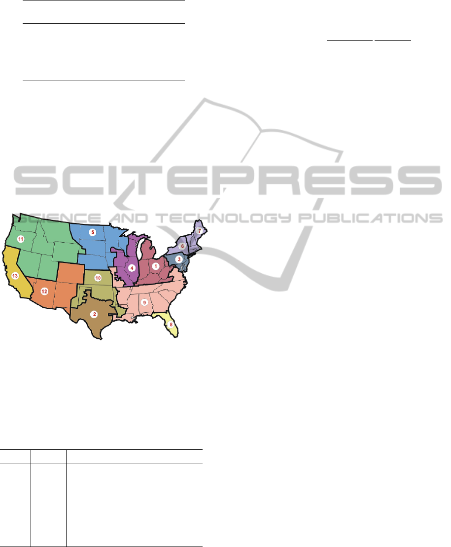
Table 2: WTT GHG emission factors for electricity genera-
tion, by fuel.
GHG (kg CO
2
eq/kWh)
f
elec
Coal 1.23
Natural Gas 0.64
Oil 1.03
Nuclear 0.02
Renewables 0.00
California. The mix for other regions was extracted
from the 2009 Annual Energy Outlook supplemental
tables (EIA, 2009), which use regions defined by the
National Energy Modeling System (NEMS) shown
in Figure 1. Using GREET’s CO
2
factors and the
AEO2009 regional electricity feedstock mix, we can
calculate the weighted average WTT CO
2
eq emis-
sion factors for a region or state. Table 3 shows the
weighted emissions factors for each region and a list
of the states included in each region.
Figure 1: Electricity generation regions used in AEO2009
and GREET 1.8d.0. GREET combines regions 3, 6, and
7 to form the Northeast region. Region names: East Cen-
tral #1, Texas #2, Northeast #3+#6+#7), Mid-America #4,
Mid-Continent #5, Florida #8, Southeast #9, OK, KS #10,
Northwest #11, CO, AZ, NM #12, and CA #13. Graphic
from (EIA, 2009).
Table 3: Regional and state electricity GHG emission fac-
tors.
Region kg CO
2
eq coal natural oil nuclear renew-
# per kWh gas ables
1 1.074 84.2% 4.7% 0.3% 10.0% 0.8%
2 0.734 36.3% 44.1% 0.1% 12.5% 7.0%
3+6+7 0.412 29.9% 21.7% 2.2% 33.9% 12.3%
4 0.728 56.2% 4.2% 0.2% 35.2% 4.2%
5 0.893 71.5% 0.8% 0.3% 14.1% 13.3%
8 0.763 34.1% 42.3% 6.6% 14.1% 2.9%
9 0.743 52.3% 13.6% 0.5% 29.4% 4.2%
10 0.990 69.0% 21.0% 0.3% 4.4% 5.3%
11 0.440 31.6% 7.6% 0.1% 3.5% 57.2%
12 0.843 51.9% 31.2% 0.1% 9.0% 7.8%
13 0.338 13.3% 36.6% 0.0% 20.5% 29.6%
US Avg 0.721 50.4% 18.3% 1.1% 20.0% 10.2%
The EPA reports fuel economy for BEVs in
MPGe, miles per gallon equivalent, based on the
based on the fact that combustion of a gallon of gaso-
line releases 121 MJ (33.7 kWh) of energy (DOE,
2000). Equation 2 is used to calculate the annual met-
ric tons of CO
2
eq emissions for a BEV operating in a
particular state.
GHGe
W TW
= V MT
f
elec,region
1000MPGe
33.7kWh
gal
, (2)
where V MT is annual travel (miles), MPGe is
the EPA label mile/gallon equivalent fuel economy,
f
elec,region
is the electricity generation emission factor
(kg CO
2
eq/kWh) for a state (Table 3), and there are
33.7 kWh/gallon of gasoline.
PHEVs operate using a combination of electricity
from the grid and internal combustion energy. PHEV
CO
2
emissions are calculated as a weighted average
of WTW CO
2
from electric mode and internal com-
bustion mode based on the shares of travel that take
place in each mode. The utility factor (λ) is the share
of travel in electric mode, often referred to as battery
charge-depleting mode. The fuel economy label pro-
vides the all-electric range (AER) in miles. Assuming
one charge per day, we estimate the annual λ as the
AER multiplied by 365 and divided by the annual to-
tal mileage. Like BEVs, the carbon intensity of elec-
tricity used by PHEVs varies by region of operation.
Equation 3 provides the annual metric tons of GHGs
emitted by a PHEV operating in a particular state.
GHGp
W TW
= λGHGe
W TW
+ (1 − λ)GHG
W TW
, (3)
where λ is the share of travel in electric (charge-
depleting) mode, GHG
W TW
from (1) is the emissions
from gasoline and GHGe
W TW
from (2) is the emis-
sions from electricity generation.
Figure 2 compares the CO
2
eq emissions of a 2012
Ford Focus, ICEV versus BEV. We can see that the
WTW emissions for the ICEV are about the same as a
BEV driven in Michigan with coal-intense electricity,
but are nearly 3 times higher than a BEV driven in
California with large shares of nuclear and renewable
electricity.
3 MATHEMATICAL MODEL
There are two main goals that we aim to achieve
in identifying fleet purchase options through opti-
mization: minimizing cost and minimizing emissions.
Rather than optimizing to obtain a single purchase
recommendation, we aim to present points from the
Pareto frontier from which customers can select their
preferred levels of sustainability and cost.
Pareto frontier visualization is a classic technique
for addressing multi-objective optimization problems.
TheParetoFrontierforVehicleFleetPurchases-CostversusSustainability
29
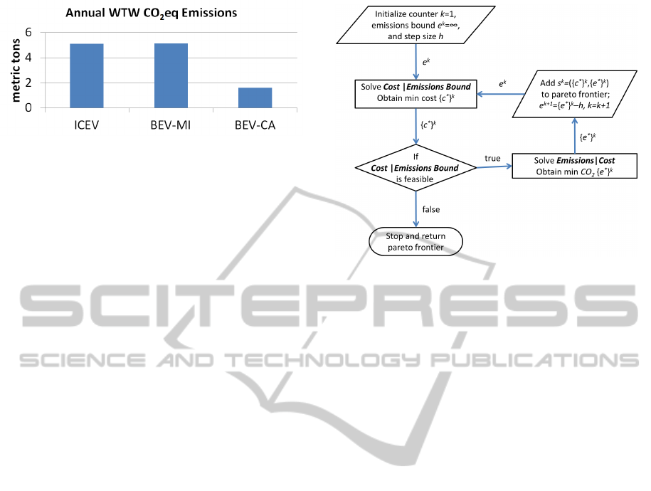
Figure 2: 2012 Ford Focus: ICEV vs BEV, 15000 miles,
55% city, Michigan (MI) and Calfornia (CA) electric grids
for BEV.
In the context of sustainability and cost, it has re-
cently been applied to supply chain network design
problems (Wang et al., 2011).
To calculate the Pareto frontier for fleet purchases,
we developed an algorithm that repeatedly solves the
following two optimization problems:
• Cost | Emissions Bound: this IP minimizes the
cost while satisfying the emissions bound e
k
,
which is initialized to ∞ and is then iteratively
reduced until the problem becomes infeasible, at
which point the algorithm terminates. The objec-
tive function value {c
∗
}
k
, is used as the required
cost in the next IP.
• Emissions | Cost: this IP minimizes the emissions
{e
∗
}
k
, by selecting the best replacement strategy
given the previously calculated cost {c
∗
}
k
. The
optimal emissions {e
∗
}
k
are then reduced by a
predetermined step size h to set the emissions
bound e
k+1
= {e
∗
}
k
− h for the next iteration.
The algorithm is outlined in Figure 3. The result
is a Pareto frontier of purchase options that include
the types and quantities of vehicles to purchase as
replacements for currently owned vehicles in a cus-
tomer’s fleet.
We define the notation that we will use to formu-
late the IPs and provide a corresponding example, de-
noted with , as follows:
• R is the set of currently owned vehicles being re-
placed.
R = {2010 Ford Fusion 3.5L - 17K miles/year
Florida, 2010 Ford Fusion 3.5L - 51K miles/year
Michigan}.
• q
r
is the number of units of vehicle r ∈ R being
replaced.
~q = [4,6].
• V is the set of vehicles available for purchase.
V = {2012 Ford Fusion 2.5L, 2012 Ford Fusion
Hybrid, etc.}.
Figure 3: Flowchart for optimizations to produce the Pareto
frontier.
• c
v
is the cost of vehicle v ∈ V (e.g. total cost of
ownership or purchase price with or without fuel
costs).
~c = [$20705,$28775, etc.] (starting MSRP price).
• V
r
⊆ V is the subset of vehicles available for pur-
chase that are suitable replacements for currently
owned vehicle r ∈ R.
V
1
= V
2
= {2012 Ford Fusion 2.5L, 2012 Ford Fu-
sion Hybrid}.
• e
v,r
is the emissions produced by vehicle v ∈ V
when replacing vehicle r ∈ R, which is a function
of the fuel economy of v and the annual mileage
of r, as described in Section 2.
e
1,1
= 6.9, e
2,1
= 4.8, e
1,2
= 20.7, e
2,2
= 14.3
(metric tons CO
2
).
• e
k
is the maximum emissions allowed at iteration
k.
e
k
= ∞ (no limit initially, to minimize price).
• F is the set of vehicle features and categories be-
ing considered, for example, moonroof, hybrid,
leather, manual, Fusion 2.5L, Focus, etc.
F = {hybrid}.
• f
l
is a lower-bound on the number of vehicles to
be purchased with feature f ∈ F.
hybrid
l
= 2.
• f
u
is an upper-bound on the number of vehicles to
be purchased with feature f ∈ F.
hybrid
u
= 8.
• f
v
is a boolean parameter that indicates whether
or not vehicle v ∈ V contains feature f ∈ F.
~
hybrid = [false, true].
ICORES2013-InternationalConferenceonOperationsResearchandEnterpriseSystems
30

The decision variables in both integer programs are
the same: x
v,r
is the number of units of vehicle v ∈ V
to purchase to replace vehicle r ∈ R.
We formulate Cost | Emissions Bound as follows:
Cost | Emissions Bound
{c
∗
}
k
= min
∑
r∈R
∑
v∈V
r
c
v
x
v,r
(4)
s.t.
∑
r∈R
∑
v∈V
r
e
v,r
x
v,r
≤ e
k
(5)
∑
v∈V
r
x
v
= q
r
∀r ∈ R (6)
f
l
≤
∑
r∈R
∑
v∈V
r
: f
v
=true
x
v,r
≤ f
u
∀ f ∈ F (7)
~x ∈ {0,1, ···}, (8)
where (4) minimizes the total purchase cost, (5) sets
the emissions limit, (6) is a flow-balance constraint
that ensures exactly one vehicle is purchased for each
vehicle being replaced, (7) provides lower and upper
bounds on features or vehicle types, and (8) requires
non-negative integer solutions for the number of ve-
hicles purchased.
Continuing our example, we first find the minimal
purchase cost with no emissions bound (e
1
= ∞), so
we have
{c
∗
}
1
=min 20705(x
1,1
+ x
1,2
) + 28775(x
2,1
+ x
2,2
)
(9)
s.t. 6.9x
1,1
+ 4.8x
2,1
+ 20.7x
1,2
+ 14.3x
2,2
≤ ∞
(10)
x
1,1
+ x
2,1
= 4 (11)
x
1,2
+ x
2,2
= 6 (12)
2 ≤ x
2,1
+ x
2,2
≤ 8 (13)
~x ∈ {0,1, ···}, (14)
where (9) minimizes purchase price, constraint (10)
that sets the initial emissions bound e
1
= ∞ is auto-
matically satisfied, constraint (11) replaces the 4 ve-
hicles in Florida, constraint (12) replaces the 6 vehi-
cles in Michigan, constraint (13) includes between 2
and 8 hybrids, and constraint (14) ensures integrality.
An optimal solution (not unique) is x
1,1
= 2, x
2,1
= 2,
x
1,2
= 6, x
2,2
= 0, which achieves the lower limit on
hybrids of 2 and thereby minimizes purchase cost.
The optimal objective value is {c
∗
}
1
= $223190. The
emissions level achieved in the left-hand side of (10)
is 147.6 metric tons of CO
2
. However, this emissions
level is not the lowest one achievable for a purchase
of 2 hybrids and 8 conventional engine vehicles. This
is why we need one more integer program that opti-
mizes emissions for a given cost.
We formulate Emissions | Cost as follows:
Emissions | Cost
{e
∗
}
k
= min
∑
r∈R
∑
v∈V
r
e
v,r
x
v,r
(15)
s.t.
∑
r∈R
∑
v∈V
r
c
v
x
v,r
= {c
∗
}
k
(16)
∑
v∈V
r
x
v
= q
r
∀r ∈ R (17)
f
l
≤
∑
r∈R
∑
v∈V
r
: f
v
=true
x
v,r
≤ f
u
∀ f ∈ F (18)
~x ∈ {0,1, ···}, (19)
where (15) minimizes emissions, (16) ensures the
purchase cost is the same as the optimal solution
{c
∗
}
k
of Cost | Emissions Bound in (4), and con-
straints (17) - (19) are the same as (6) - (8). The result-
ing s
k
= ({c
∗
}
k
,{e
∗
}
k
) is added to the Pareto frontier,
and the value for e
k+1
is reduced to {e
∗
}
k
− h, where
h is a predetermined step size.
Continuing our example, we have
{e
∗
}
1
= min 6.9x
1,1
+ 4.8x
2,1
+ 20.7x
1,2
+ 14.3x
2,2
(20)
s.t. 20705(x
1,1
+ x
1,2
) + 28775(x
2,1
+ x
2,2
) = 223190
(21)
x
1,1
+ x
2,1
= 4 (22)
x
1,2
+ x
2,2
= 6 (23)
2 ≤ x
2,1
+ x
2,2
≤ 8 (24)
~x ∈ {0,1, ···}. (25)
The optimal solution (unique) is x
1,1
= 4, x
2,1
=
0, x
1,2
= 4, x
2,2
= 2. While the same vehi-
cles are purchased as in Cost | Emissions Bound,
the optimal emissions level achieved of {e
∗
}
1
=
139 metric tons of CO
2
is 6% lower; this emis-
sions reduction emphasizes the importance of plac-
ing the vehicles optimally. s
1
= ({c
∗
}
1
,{e
∗
}
1
) =
($223190,139 metric tons CO
2
) is added to the
Pareto frontier, and the value for e
2
is reduced to
138 metric tons CO
2
, where the step size is h =
1 metric ton CO
2
.
We continue our algorithm to compute the sec-
ond point in the Pareto frontier by substituting e
2
=
138 metric tons CO
2
into the right-hand side of con-
straint (10) and resolving Cost | Emissions Bound.
An optimal solution (again not unique) is x
1,1
= 1,
x
2,1
= 3, x
1,2
= 6, x
2,2
= 0, which includes 3 hybrids.
This is the minimum number of hybrids that can be
purchased while satisfying the emissions bound of
138 metric tons CO
2
. The optimal objective value is
{c
∗
}
2
= $231260. The emissions level achieved in
the left-hand side of (10) is 145.5 metric tons of CO
2
.
Similarly to the first iteration (k = 1), this emissions
TheParetoFrontierforVehicleFleetPurchases-CostversusSustainability
31
level is not the lowest one achievable for a purchase
of 3 hybrids and 7 conventional engine vehicles.
To find the emissions level for the second point
in the Pareto frontier, we substitute {c
∗
}
2
= $231260
into the right-hand side of constraint (21) and resolve
Emissions | Cost. The optimal solution (unique) is
x
1,1
= 4, x
2,1
= 0, x
1,2
= 3, x
2,2
= 3. While the same
vehicles are purchased as in Cost | Emissions Bound,
the optimal emissions level achieved of {e
∗
}
2
= 132.6
metric tons of CO
2
is 9% lower. The resulting s
2
=
({c
∗
}
2
,{e
∗
}
2
) = ($31260, 132.6 metric tons CO
2
) is
added to the Pareto frontier, and the value for e
3
is
reduced to 131.6 metric tons CO
2
.
The algorithm, summarized in Figure 3, continues
to iteratively solve the Cost | Emissions Bound and
Emissions | Cost IPs for k = 3, 4,5, 6,7 to provide us
with additional points s
3
,s
4
,s
5
,s
6
,s
7
. At k = 8, no
further emissions reductions are achievable due to the
limit of 8 hybrids, which yields an infeasible Cost |
Emissions Bound IP, and the algorithm terminates.
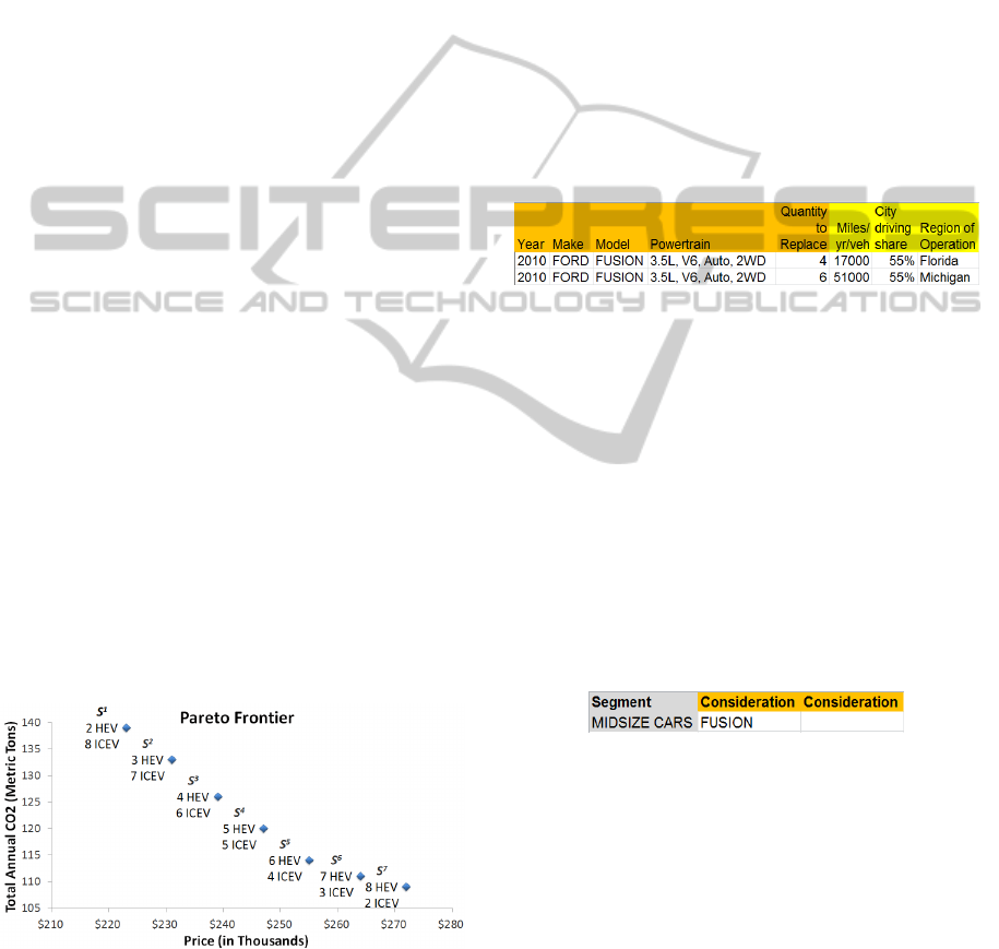
The Pareto frontier for this example in Figure 4
shows solutions for all iterations k = 1,. .. ,7. These
solutions describe which combinations of vehicles
to purchase to replace the 10 vehicles: the solution
varies between 2 and 8 HEVs and ICEVs. While the
points in Figure 4 are spaced evenly with respect to
price, the CO
2
reductions become smaller when 7 and
8 HEVs are chosen for purchase; this can be explained
by the higher mileage on the 6 Michigan vehicles,
where hybrids are first optimally placed, compared
with the lower mileage of the Florida vehicles, where
HEVs 7 and 8 are placed. This example is sufficiently
concise to solve with logic and intuition alone; with
large fleets containing vehicles with variable mileage
and more vehicles considered as candidate replace-
ments, the Pareto frontier is quite useful in identifying
strategic purchase decisions.
Figure 4: The Pareto frontier.
While we have concentrated on formulations that
minimize purchase price in this section, additional ob-
jectives are also useful in practice; two such notewor-
thy objectives are minimizing purchase price plus fuel
costs for a given number of years and minimizing to-
tal cost of ownership.
4 SOFTWARE APPLICATION
We have developed a Microsoft Excel user interface
for the Fleet Purchase Planner. Fleet customers up-
load information on their current fleets to the tem-
plate shown in Figure 5. Data collected includes year,
make, model, and powertrain, which are mapped to
EPA fuel economy data. Combining this with annual
mileage, city driving share, and region of operation,
we calculate the current state CO
2
, as described in
Section 2. The input for “quantity to replace” in Fig-
ure 5 is used to generate the flow-balance constraints
(6), (11), (12), (17), (22) and (23).
Figure 5: Input for the set of vehicles being replaced, R,
from the example in Section 3.
To determine candidate replacements V
r
for those
vehicles r ∈ R listed in Figure 5, we use vehicle seg-
mentation data. For example, we look up “2010 Ford
Fusion 3.5L, V6, Auto, 2WD” in our segmentation
database and find that this is a midsize car. We then
refer to the spreadsheet user interface in Figure 6,
which lists Fusion as a suitable candidate replacement
for midsize cars. This interface offers the flexibility
to list multiple candidate replacements, so customers
can explore various options; for example, the choice
for replacement vehicles could move down in size to
a compact car or up to a crossover utility vehicle.
Figure 6: Segmentation lookup table for vehicles available
for purchase.
The interface in Figure 6 is used to narrow down
the subset of candidate replacements V
r
from all Ford
vehicles to all Fusion vehicles. However, in the exam-
ple from Section 3, we considered only two Fusion
vehicles as a candidate replacements: the automatic
2.5L ICEV and the HEV. In practice, we achieve this
through our feature sets F and constraints (7) and
(18). The information required to generate these con-
straints is input by the user in the spreadsheet inter-
face shown in Figure 7. For example, a maximum of
0 ”Manual” removes manual transmission Fusion ve-
hicles from consideration. This is also where we in-
ICORES2013-InternationalConferenceonOperationsResearchandEnterpriseSystems
32
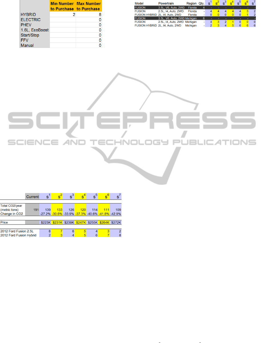
Figure 7: Upper and lower limits, f
l
and f
u
, respectively, on
the features and categories, f ∈ F, for vehicles available for
purchase.
troduce the range of 2 to 8 HEVs for constraints (13)
and (24).
The analytical engine for the Fleet Purchase Plan-
ner is implemented in Java and CPLEX 12.4 is used
to solve the IPs. These IPs are easily solved for fleets
with up to several thousand vehicles, with solve times
under 1 second on an Intel Core i5 2.5 GHz CPU with
8GB RAM running 64 bit Windows 7.
In addition to the Pareto frontier shown in Figure
4, there is other information that could be useful to the
customer. The report shown in Figure 8 highlights the
improvement in sustainability corresponding to each
point on the Pareto frontier compared with the current
state of the fleet. This report may also include com-
parisons of fuel expenditure over a given time period
versus purchase price, further illustrating the relation-
ship between cost and sustainability.
Figure 8: Summary report for multiple purchase options
corresponding to points s
1
,·· · , s
7
on the Pareto frontier.
The second report in Figure 9, provides the opti-
mal placement of each vehicle purchased for the var-
ious scenarios. It can also include summary statistics
for annual fuel expenditure and CO
2
emissions on the
individual vehicle level, compared to the current level
for the vehicle being replaced. Each new vehicle be-
ing purchased appears below the vehicle it is replac-
ing. Notice that in the min cost scenario s
1
, the two
HEVs purchased replace the higher mileage vehicles
in Michigan. As the upper bound on emissions e
k
is
lowered at each iteration k, more vehicles in Michigan
are replaced with HEVs. Only after all the Michigan
vehicles have been replaced with hybrids, at s
5
, is a
vehicle in Florida replaced with a hybrid.
Figure 9: Detailed report for multiple purchase options cor-
responding to points s
1
,·· · , s
7
on the Pareto frontier. The
vehicles being replaced are shown with a black background
and white font, with their corresponding replacements be-
low.
5 CONCLUSIONS
Ford’s Fleet Purchase Planner is a software system
designed to identify the most cost effective opportu-
nities for vehicle fleets to improve their sustainability
through new purchases. FPP leverages several data
sources, including vehicle fuel economy, segmenta-
tion, customers’ current fleets and driving patterns.
The IP models we have introduced generate the Pareto
frontier, which demonstrates the relationship between
cost and sustainability. This technology, for the first
time, provides customers with current emissions lev-
els of their vehicle fleets and compares that with levels
achieved by various purchase options.
FPP has already been used in collaboration with
large fleet customers, with significant demonstrated
financial benefits over more traditional vehicle re-
placements strategies. For example, one such strat-
egy is to select a single new midsize vehicle, such as
a Ford Fusion EcoBoost, to purchase for any midsize
vehicle being replaced. We can show the minimum
cost purchase to achieve the same level of sustainabil-
ity using the Pareto frontier, thereby highlighting the
value of optimization.
FPP has the potential to change the way many of
Ford’s fleet customers plan their purchases, and more
importantly, the decisions they make regarding what
to purchase.
REFERENCES
DOE (2000). Electric and hybrid vehicle research, de-
velopment, and demonstration program: Petroleum-
equivalent fuel economy calculation. Technical report,
Federal Register 65, 113, 36986.
EIA, U. (2009). Annual energy outlook 2009 with projec-
tions to 2030. Technical report, DOE/EIA-0383.
Ford Motor Company (2010a). Kraft foods to re-
place U.S. sales fleet. http://media.ford.com/
article
display.cfm?article id=32202.
Ford Motor Company (2010b). Simplexgrinnell or-
ders 200 ford fusion hybrids in effort to reduce
TheParetoFrontierforVehicleFleetPurchases-CostversusSustainability
33

greenhouse gas emissions. http://media.ford.com/
article display.cfm?article id=32710.
Ma, H., Balthasar, F., Tait, N., Riera-Palou, X., and Harri-
son, A. (2012). A new comparison between the life
cycle greenhouse gas emissions of battery electric ve-
hicles and internal combustion vehicles. Energy Pol-
icy.
Notter, D., Gauch, M., Widmer, R., W
¨
ager, P., Stamp, A.,
Zah, R., and Althaus, H. (2010). Contribution of li-
ion batteries to the environmental impact of electric
vehicles. Environmental science & technology.
Solomon, S. (2007). Climate change 2007: the physical
science basis: contribution of Working Group I to
the Fourth Assessment Report of the Intergovernmen-
tal Panel on Climate Change. Cambridge University
Press.
Wang, F., Lai, X., and Shi, N. (2011). A multi-objective
optimization for green supply chain network design.
Decision Support Systems, 51(2):262–269.
Wang, M. (1999). Greet 1.5-transportation fuel-cycle
model-vol. 1: methodology, development, use, and
results. Technical report, Argonne National Lab., IL
(US).
ICORES2013-InternationalConferenceonOperationsResearchandEnterpriseSystems
34
