
Curvature-Scale-based Contour Understanding for Leaf
Margin Shape Recognition and Species Identification
∗
Guillaume Cerutti
1,2
, Laure Tougne
1,2
, Didier Coquin
3
and Antoine Vacavant
4
1
Universit´e de Lyon, CNRS, Lyon, France
2
Universit´e Lyon 2, LIRIS, UMR5205, F-69676, Lyon, France
3
LISTIC, Domaine Universitaire, F-74944, Annecy le Vieux, France
4
Clermont Universit´e, Universit´e d’Auvergne, ISIT, F-63001, Clermont-Ferrand, France
Keywords:
Curvature-Scale Space, Contour Characterization, Leaf Identification, Shape Classification.
Abstract:
In the frame of a tree species identifying mobile application, designed for a wide scope of users, and with
didactic purposes, we developed a method based on the computation of explicit leaf shape descriptors inspired
by the criteria used in botany. This paper focuses on the characterization of the leaf contour, the extraction
of its properties, and its description using botanical terms. Contour properties are investigated using the
Curvature-Scale Space representation, the potential teeth explicitly extracted and described, and the margin
classified into a set of inferred shape classes. Results are presented for both margin shape characterization,
and leaf classification over nearly 80 tree species.
1 INTRODUCTION
Plants, trees and herbs that used to constitute the
most immediate environment for past generations,
seem somehow disconnected from our everyday life,
in a world of rampant urbanization and invasive
technology. Knowledge of the uses and properties of
numerous species got away, kept only by a handful of
botanists. Even identifying a simple plant has merely
become a case for the specialists.
But the blossoming of mobile technology
curiously offers the opportunity of spreading back
this knowledge into everyone’s pocket. Providing
an intuitive and flexible way to recognize species,
to teach anyone who feels the need how to look at a
plant, is now a possibility. Attempts in this direction
have come to light with great success, being with
user-based (TreeId, Fleurs en Poche) or automatic
recognition (LeafSnap
1
) on white background
images.
Leaves are a choice target for such application,
present almost all year long, easy to photograph, and
∗
This work has been supported by the French National
Agency for Research with the reference ANR-10-CORD-
005 (REVES project).
1
http://leafsnap.com : developed by researchers from
Columbia University, the University of Maryland, and the
Smithsonian Institution (Belhumeur et al., 2008)
with well studied geometrical specificities that make
the identification, if not trivial, possible. Our main
objective is to build a system for leaf shape analysis
of photographs in a natural environment, relying on
high-level geometric criteria inspired by those used
by botanists to classify a leaf into a list of species.
In this paper, we focus on the characterization
of the leaf margin shape, introducing a dedicated
description of the shape contour. Section 2 presents
works connected to this matter. The processing
performed on the contour is described in Section
3 and the descriptor we use detailed in Section
4. Section 5 expounds its interest for both margin
shape classification and species identification, and
conclusions are drawn in Section 6.
2 RELATED WORKS
2.1 Leaf Identification
Leaf image retrieval and plant identification have
been a growing topic of interest in the past few
years. Some authors (Belhumeur et al., 2008) also
aim at conceiving a mobile guide, achieving great
performance on plain background images by the
277
Cerutti G., Tougne L., Coquin D. and Vacavant A..
Curvature-Scale-based Contour Understanding for Leaf Margin Shape Recognition and Species Identification.
DOI: 10.5220/0004225402770284
In Proceedings of the International Conference on Computer Vision Theory and Applications (VISAPP-2013), pages 277-284
ISBN: 978-989-8565-47-1
Copyright
c
2013 SCITEPRESS (Science and Technology Publications, Lda.)

combination of established shape descriptors (Inner-
Distance Shape Context) and classification methods.
Some works tackle the challenge of segmentation
over natural background (Teng et al., 2009; Wang
et al., 2008), but most elude this obstacle, working on
plain background images, where sensitivity to noisy
shapes is less of an issue given the general accuracy
of the obtained contours.
Many methods rely on statistical features such as
moments (Wang et al., 2008), histogram of gradients
or local interest points (Go¨eau et al., 2011b) or
generic contout descriptors such as the Curvature-
Scale Space (Mokhtarian and Abbasi, 2004). Such
descriptors were not designed to take into account
the nature of the object, but fit quite well with
its specificities. A commonly used geometrical
descriptor for leaf image retrieval is the Centroid-
Contour Distance (CCD) curve (Wang et al., 2000;
Teng et al., 2009) though it can be applied to any type
of object.
On the other hand, some morphological features
explicitly computed on the shape of the object to
model its natural properties have also been used (Du
et al., 2007; Go¨eau et al., 2011b). Even more
dedicated methods have been designed, basing their
recognition on an explicit representation of the leaf
contour and of its teeth (Im et al., 1998; Caballero and
Aranda, 2010) but suitable only for image retrieval
and applied to a small number of species.
2.2 Curvature for Contour Description
Since the leaf margin shape is a very discriminant
feature for identification, characterizing the contour
of the leaf is a crucial step. The CCD curve provides
an interesting view, but lacks precision, as the curve
for a leaf with small teeth will be very close to a
smooth one. To discriminate such contours, the use
of curvature is very advantageous.
A rich representation of the contour is the
Curvature-Scale Space (CSS), that has already been
used in the context of shape recognition (Mokhtarian
and Mackworth, 1992) and even leaf image retrieval
(Mokhtarian and Abbasi, 2004; Caballero and
Aranda, 2010). It piles up curvature measures at
each point of the contour over successive smoothing
scales, summing up the information into a map where
concavities and convexities clearly appear.
Curvature has also been used to detect dominant
points on the contour, and provide a compact
description of a contour by its curvature optima.
This is a well studied problem (Teh and Chin,
1989) in which the introduction of the curvature-scale
transform has proved to be beneficial (Pei and Lin,
1992). The detection and characterization of salient
features on a leaf contour is a problem that can be
addressed with a similar perspective.
3 CONTOUR INTERPRETATION
Our starting point is a segmented leaf, from either
a plain or natural background, along with its
preliminary global shape estimation (Cerutti et al.,
2011). This polygonal model conveys interesting
information on the leaf’s geometry, and provides
notably the number of appearing lobes n
L
and an
estimation of its main axis (possibly more than one
in the case of a palmately lobed leaf). Our frame
of work here comprises only simple and palmately
lobed leaves (nearly 75% of all European tree specie)
species with compound leaves being left aside. Since
our goal is to represent the morphologyof the margin,
knowing where to look is important to select the
accurate features and, for instance, not consider the
apex as a simple tooth.
3.1 Leaf Contour Partition
The contour needs then to be divided into areas
corresponding to the apex, to the base, to the potential
lobe tips, and finally to the rest of the margin, so that
the most salient features do not absorb the rest of the
information. Relying on the polygonal leaf model is
here useful to solve what would otherwise be a much
more complicated task. Supposing that the axes of
the polygonal model are accurate, we can use them to
mark off contour points that are in one of these areas
of interest.
Figure 1: Polygonal model and labelling of contour parts
corresponding to leaf areas.
To achieve the labelling shown in Figure 1, we
define sets of vertices as the intersection of the
contour with a fixed angular sector, built around the
corresponding axis using the model points, issuing
from the opposite point (base for the apices, and apex
for the base) and with a minimal distance relatively to
this point : A for the apical area (red), B for the basal
VISAPP2013-InternationalConferenceonComputerVisionTheoryandApplications
278

area (blue), L for the lobe tips (brown), and the actual
margin area M , divided into for lM the left margin
area and rM for the left margin area (green).
This partition first makes possible the accurate
location of the actual base point
ˆ
B and the apex
point
ˆ
A of the leaf, as the most salient features in
their respective area B or A , a crucial information
to estimate the local shape of the leaf around them,
a determining feature for botanists. And secondly,
outside of these areas, we can study the properties
of potential teeth, lobes, sinuses and other salient
features in M , and characterize the leaf margin shape,
and only it.
3.2 Curvature-Scale Space Transform
As a matter of fact, the salient features on the contour
appear very clearly on the Curvature-Scale Space
transform of the contour, as shown in Figure 3(b).
The CSS is a very powerful description but is too
informative to be used as a descriptor and to build
class models by averaging several of them. As we
wish to locate and characterize precisely curvature-
defined elements on the contour, it was a more
judicious choice to look, not at zero-curvature points
as the original method would do (Mokhtarian and
Mackworth, 1992), but on the contrary at the maxima
and minima of curvature. These salient points are
the ones that visually stand out in the CSS image and
can be intuitively be matched to existing structures on
the leaf contour, reason why we want to detect them
explicitly.
3.3 Detecting Teeth and Pits
To locate these points, we actually want to detect
dominant points on the leaf contour and to find the
scale of the concave or convex part they correspond
to. The method we use is largely inspired of existing
works (Teh and Chin, 1989; Pei and Lin, 1992) where
the process of detection is performed at each scale
level. Starting with S = 4 (lower scale elements being
arguably indiscerniblefrom noise) the set of dominant
points at each scale D(S) is initialized with all the
contour points and the process is then the following:
1. Extract points for which the curvature value is a
local optimum in a neighbourhood of size S
2. Suppress points the curvature intensity of which
is below a threshold k
min
3. Suppress points that can not be traced to a
dominant point at the previous scale (if S > 4)
4. Keep only the medianpoint of potentialremaining
groups of size ≤ S
The result we obtain is a map of the located
dominant points at each scale, as presented in Figure
3(c). This representation reveals the teeth and pits of
the contour in the form of chains of dominant points.
4 LEAF MARGIN DESCRIPTION
Once the salient features are detected on the contour,
it is necessary to interpret this dense information in
order to make the discriminant characteristics of the
margin appear. To know what to look for, we relied
on the distinctions made by botanists to discriminate
the different species.
4.1 Leaf Margin Shapes in Botany
To describe the shape of the leaf margin, botanists
use a terminology that refers both to the properties
of teeth taken separately and to their repartition over
the margin. Some of these terms are shown in Figure
2. For instance a ”doubly serrate” leaf implies two
levels of teeth with different sizes and frequencies,
with bigger teeth divided into smaller sub-teeth. The
words themselves are vague enough so that leaves
with teeth that look rather different may fall inside
the same term.
Figure 2: Examples of leaf margin shapes : Entire,
Denticulate, Dentate, Sinuate, Lobate. Images taken from
(Coste, 1906).
The margin shape constitutes however a very
discriminant criterion for species identification that
generally presents less variability than the global
shape, with the exception of some pathological
species. Our descriptor will have to capture the
differences regarding size, sharpness, orientation,
repartition and variability of the teeth implied in the
botanical terms, but also to benefit from the use of
numerical values to be more precise and discriminate
leaves of different aspect that would be called the
same.
4.2 Margin Interpretation
For the sake of interpretation, we want to use the
representation of the contour by dominant points to
retrieve the properties of every located structure on
Curvature-Scale-basedContourUnderstandingforLeafMarginShapeRecognitionandSpeciesIdentification
279

(a) (b) (c)
Figure 3: Traced dominant points over scale (c) and their curvature, obtained from the curvature-scale space transform (b) of
a leaf contour (a).
the contour. Each chain that appears on the dominant
points map corresponds indeed to a convex or a
concave part, and its actual size, as a human eye
would interpret it, is the scale until which it persists,
that is to say the scale of the chain’s end point.
We scan the dominant points starting from the
highest scale to keep only these terminal points.
When a dominant point is found at scale S, all the
dominant points of the same curvature sign are simply
suppressed at lower scales, in a neighbourhood of
size S. This way, we ensure that a single structure
is not counted twice, and small structures which are
included in larger ones are merged into one.
Each point kept after this selection step
corresponds to a concave or convex structure of
scale S. To complete this size information, we
estimate the actual curvature
¯
K of a dominant point
of scale S belonging to D(S), as the average curvature
of all the dominant points belonging to the same
chain. This computation is done while suppressing
the points at lower scales.
(a) (b) (c)
Figure 4: Various leaf contours with detected base, apex,
teeth and pits; apex area in red, base area in dark
blue; convexities in orange, concavities in blue, brightness
representing curvature intensity, extent representing scale.
Finally the final set of dominant points is a
semantically rich interpretation of the leaf contour,
where the base and apex points
ˆ
B and
ˆ
A are
precisely located, and where teeth are detected and
characterized independently in terms of position on
the contour (u), size (S) and curvature (K) : each point
p in then represented by a vector (u(p);S(p);K(p)).
This representation is displayed in Figure 4.
To improve robustness, and avoid that errors
in segmentation or unwanted leaf artefacts (cracks,
holes, spots) are taken into account, we want to keep
only points that can be found on both sides of the
leaf. Here again, the contour partition is very useful
to know on which side lies a given point, and where
to look on the contour to know if a similar one exists
on the opposite side. The matching is performed by
computing a distance term to all the points on the
opposite side of same curvature sign, that takes into
account their scale, curvature, relative position on the
axis
ˆ
B
ˆ
A
, and relativedistance to this same axis. This
method is somewhat risky but ensures that eccentric
structures as in Figure 5 do not bias the understanding
of the margin.
Figure 5: Suppression of points that can not be matched on
a deteriorated leaf ; only connected points are kept.
4.3 Describing the Margin
Even if this explicit representation is full of
information and could be used as such to compare
two leaves, it is still too heavy if we want to average
several of them for classification purposes. It is
necessary to sum it up into a condensed descriptor to
capture the main properties of the margin, and allow
a semantic interpretation of its specificities.
A first characterization consists in measuring how
much of the leaf margin is convex, concave or neither
of the two. Since the detected structures, given their
VISAPP2013-InternationalConferenceonComputerVisionTheoryandApplications
280

definition, account for a number of vertices equal
to their scale, we just have to sum the scales of
dominant points and normalize them, to compute 3
parameters w
+
, w
−
and w
0
, corresponding to the
percentageof the set M of margin verticesthat belong
respectively to convex structures, concave structures,
and no structure.
To describe teeth properties in a condensed way,
we compute averages and standard deviations for the
properties we extracted on each dominant point. That
gives 8 parameters computed on either concave (-) or
convex (+) points, respectively
¯
S
+
, σ
S+
,
¯
S
−
, σ
S−
for
scale, and
¯
K
+
, σ
K+
,
¯
K
−
, σ
K−
for curvature. These
values are computed by weighting the considered
parameter of each point by the point’s scale, so that
each vertex on the margin contributes at the same
level.
Even if computing standard deviations provide a
measure for the variability of the properties, such
aggregating representation constitute a loss of spatial
information. To keep a trace of the repartition of teeth
along the margin, we computed the relative distances
d ↑ (p) and d ↓ (p) of each point p, respectively to the
next and previous points of opposite curvature on the
same side M (p), when they exist.
These distances are once again averaged over
points of the same curvature sign to produce 4
additional parameters
d ↑
+
, d ↓
+
for convex points,
and
d ↑
−
, d ↓
−
for concave points, that account for
the spatial repartition of teeth on the margin. What
we finally use to describe the margin is a vector P of
11 parameters :
•
¯
S
+
+ σ
S+
•
¯
S
+
− σ
S+
•
¯
K
+
+ σ
K+
•
¯
K
+
− σ
K+
•
¯
S
−
+ σ
S−
•
¯
S
−
− σ
S−
•
¯
K
−
+ σ
K−
•
¯
K
−
− σ
K−
• w
0
•
d ↑
+
/d ↓
+
•
d ↑
−
/d ↓
−
Taken together, these parameters constitute a
very condensed yet efficient representation of what
is important on a leaf contour, summing up the
properties a botanist would investigate to characterize
the margin. Most of the computational time comes
from the CSS transform, but can be greatly reduced
by computing only a limited number of scales and
interpolating the curvature value for intermediate
scales, leading to an execution time below the second
on a computer processor, and of nearly 3 seconds on
an iPhone 4 processor.
5 CLASSIFICATION & RESULTS
To assess the relevance of our margin descriptors, we
chose to classify leaves in botanical terms. However,
it is impossible to have a database of leaves labelled
with their exact shapes because of the intra-species
variability and the subjectivity and vagueness of those
words. The only way to learn automatically these
shapes was to train a semi-supervised classifier using
the possible shapes for each species and let it infer the
concept represented by the classes.
5.1 Learning Margin Shapes
As a matter of fact, trying to evaluate the concepts
behind the botanical words without exactly labelled
examples is a very challenging issue. Those words
maybe used to cover different shapes that may share
some properties but not all of them. The method
we used to learn these concepts tries to consider
both the theoretical knowledge on leaf shapes and the
uncertainty on the correspondence of one given leaf
to one particular class.
Each considered species s was labelled with one
or more possible margin shapes M(s), according to
a reference botanical description (Coste, 1906). We
retained 12 terms that were applicable to all the
species we considered, namely :
• Entire
• Denticulate
• Undulate
• Crenate
• Serrate
• Dentate
• Doubly Serrate
• Sinuate
• Spiny
• Angular
• Lobate
• Pinnatifid
Then we used a semi-supervised Fuzzy C
Means (FCM) clustering algorithm to learn the
12 centroids representing the shapes. Each
individual i in the database of species s(i) is
represented by a descriptor vector P
i
= (P
k,i
)
k=1..K
and is assigned a membership value (µ
m,i
)
m=1..12
representing its degree of belonging to each of the
clusters. The supervising here consists of a constraint
that the membership of an individual to clusters
corresponding to shapes outside of the possible
shapes M(s(i)) of its species must remain zero:
∀i,∀m = 1..12,m /∈ M(s(i)) =⇒ µ
m,i
= 0. The initial
membership values are set to be the same for each
possible shape of the species, and the centroids are
then computed following the regular FCM procedure,
with a parameter β set to 1.8.
Each class is finally represented by its resulting
centroid C
m
and by the estimated standard deviation
vector Σ
m
, computed using the memberships of each
Curvature-Scale-basedContourUnderstandingforLeafMarginShapeRecognitionandSpeciesIdentification
281

individual. A new leaf, represented by its margin
parameter vector P = (P
k
) is then classified by
computingits normalized Euclidean distance to all the
class centroids, and assigning it to the closest.
5.2 Species Identification
The database used to test our algorithms is a subset
of the Pl@ntLeaves (Go¨eau et al., 2011a) database,
keeping only 5668 leaf images (out of 8422) on white,
plain or natural backgrounds of 80 species (out of
126) with non-compound leaves.
Parameters extracted on the images, outside of
the margin descriptors described here [CS], are
parameters from the polygonal leaf model [MP]
(Cerutti et al., 2011) accounting for the global shape
of the leaf, and parameters of Bezier curves based
basal and apical shape models [B/A] estimated around
the located points
ˆ
B and
ˆ
A.
The data formed by all the parameters from
all the images is first centered and normalized.
Assuming that each parameter simply follows a
Gaussian distribution, we compute class centroidsand
standard deviations with examples from the training
dataset. For each species s, and for each possible
number of lobes n
L
up to 3 we build a class Φ
s,n
L
=
(µ
s,n
L
,k
,σ
s,n
L
,k
) if at least 10% of all the species
examples have this value.
To classify a new example, we will simply have
to compare its descriptors with the centroids of the
classes sharing the same number of lobes n
L
. For
each one of the 3 sets of parameters, we compute
a Euclidean distance to the surface of the ellipsoid
defined by means and standard deviations:
D(P,Φ
s,n
L
) =
P− µ
S,n
L
2
max
1−
1
kP− µ
S,n
L
k
M
,0
kP− µ
S,n
L
k
M
=
s
∑
k
(P
k
− µ
s,n
L
,k
)
2
σ
s,n
L
,k
2
Each one of these terms is then weighted
differently after having learned the classes, dividing
it by the average distance of the correct class over
the training base, which weights it accordingly to
its significance. The final distance we use for
classification is simply the sum of these weighted
terms, and the classes are then ordered accordingly
to their distance, producing an ranked list of species.
5.3 Experimental Results
To evaluate the classification into botanical shapes,
we performed a cross validation on the training base,
learning the classes by FCM on two thirds of the
database, and classifying the remaining third. A
classification is assessed to be correct if the returned
shape is one of the possible shapes taken by the leaf
species. Results show a correct classification in 65%
of cases, climbing up to 76% if we take into account
the two first ranked classes.
We tried to refine this evaluation by building a
confusion matrix for the shapes. It is not an easy
task since the examples are not labelled by their
actual shape, but by their species and thus their
possible shapes. We decided to put a weight of 1
per example in the matrix, placing it in the diagonal
cell if the classification was considered as correct, and
splitting it among the theoretical possible classes in
the recognized class column if not. The percentages
are then obtained by dividing those weights by the
total weight of each theoretical class.
Table 1: Confusion Matrix for Leaf Margin Classification.
The matrix we obtain is displayed in Table 1 and
provides a good light on what our descriptors are
good at discriminating or not. It appears clearly
that margins with larger structures are easier to
differentiate than smaller ones. It is difficult to
capture the differences between for instance Serrate
and Dentate leaves especially since the small scale we
are looking at makes errors more common. Dentate
is visibly a very variable class, making it more easily
detected giventhe classification distance we use. Very
small teeth of Denticulate leaves seem also hard to
represent, such leaves being regularly seen as without
teeth or with regular ones.
Concerning the species classification, results
were evaluated following the same cross validation
process. We computed classification rates for
the different types of images in the Pl@ntLeaves
VISAPP2013-InternationalConferenceonComputerVisionTheoryandApplications
282
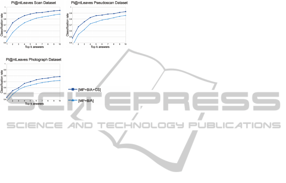
Database (Scan, Pseudoscan and Photograph) and
measured the presence of the true species among the
top k answers (k going from 1 to 10) returned by the
classification algorithm.
(a) (b)
(c)
Figure 6: Classification rates on the Pl@ntLeaves Database
on scan (a) pseudoscan (b) and photograph (c) images
Figure 6 presents the results obtained with
the global, base and apex shape descriptors only
[MP+B/A] and with the addition of the margin
descriptors [MP+B/A+CS], underlining the interest
of considering the contour in a very specific way,
with an average recognition score of 53%, and a
presence of the correct species in the 5 first answers
of 85%. The great improvement induced by the use
of curvature-based descriptors is here clearly visible.
The enhancement is less important on photographs
given the hardness of the task of retrieving the
exact leaf contour, which obviously deteriorates the
relevance of the contour description.
These scores may be compared to the results of
the 2011 ImageCLEF Plant Identification task (Go¨eau
et al., 2011a) concerning a very similar database, and
where the best participants reached an average score
of 45%.
6 CONCLUSIONS
The method presented in this article constitutes an
interesting step towards an explicative system of leaf
classification for an independent mobile application.
Being able to place high-level semantic concepts over
the values extracted from an image gives the user a
feedback that may prove of great usefulness for both
interactive and educational purposes.
A first implementation of the recognition process
on mobile devices is engaged with very satisfactory
results, but not yet with the nearly 150 native
European tree species we aim at recognizing. With
the number of potential classes increasing, it will
become a necessity to reduce the scope of the search,
by including geographical information linked to the
GPS system present in every smartphone. Knowing
in advance which species are likely to be found in
the geographical area where the user stands may be
a decisive step towards a truly reliable identification.
However, what we have now is a good base
structure for a new tree identification application,
designed to be functional in a natural environment,
and destined to anyone with interest in plants
but without the otherwise compulsory botanical
background.
REFERENCES
Belhumeur, P., Chen, D., Feiner, S., Jacobs, D., Kress,
W., Ling, H., Lopez, I., Ramamoorthi, R., Sheorey,
S., White, S., and Zhang, L. (2008). Searching the
world’s herbaria: A system for visual identication of
plant species. In ECCV.
Caballero, C. and Aranda, M. C. (2010). Plant
species identification using leaf image retrieval. In
Proceedings of the ACM International Conference on
Image and Video Retrieval, CIVR 2010, pages 327–
334.
Cerutti, G., Tougne, L., Mille, J., Vacavant, A., and Coquin,
D. (2011). Guiding active contours for tree leaf
segmentation and identification. In CLEF Working
Notes.
Coste, H. (1906). Flore descriptive et illustr´ee de la France
de la Corse et des contr´ees limitrophes.
Du, J. X., Wang, X. F., and Zhang, G.-J. (2007). Leaf shape
based plant species recognition. Applied Mathematics
and Computation, 185:883–893.
Go¨eau, H., Bonnet, P., Joly, A., Boujemaa, N., Barthelemy,
D., Molino, J.-F., Birnbaum, P., Mouysset, E., and
Picard, M. (2011a). The clef 2011 plant images
classification task. In CLEF Working Notes.
Go¨eau, H., Joly, A., Yahiaoui, I., Bonnet, P., and Mouysset,
E. (2011b). Participation of inria & pl@ntnet to
imageclef 2011 plant images classification task. In
CLEF Working Notes.
Im, C., Nishida, H., and Kunii, T. L. (1998). A hierarchical
method of recognizing plant species by leaf shapes. In
MVA, pages 158–161.
Mokhtarian, F. and Abbasi, S. (2004). Matching
shapes with self-intersections: Application to leaf
classification. IEEE IP, 13(5):653–661.
Mokhtarian, F. and Mackworth, A. (1992). A theory of
multiscale, curvature-based shape representation for
planar curves. IEEE PAMI, 14:789–805.
Pei, S. C. and Lin, C. N. (1992). The detection of
dominant points on digital curves by scale-space
filtering. Pattern Recognition, 25(11):1307–1314.
Curvature-Scale-basedContourUnderstandingforLeafMarginShapeRecognitionandSpeciesIdentification
283

Teh, C. H. and Chin, R. T. (1989). On the detection
of dominant points on digital curves. IEEE PAMI,
11(8):859–872.
Teng, C.-H., Kuo, Y.-T., and Chen, Y.-S. (2009). Leaf
segmentation, its 3d position estimation and leaf
classification from a few images with very close
viewpoints. In ICIAR, pages 937–946.
Wang, X. F., Huang, D. S., Du, J. X., Huan, X., and Heutte,
L. (2008). Classification of plant leaf images with
complicated background. Applied Mathematics and
Computation, 205(2):916–926.
Wang, Z., Chi, Z., Feng, D., and Wang, Q. (2000). Leaf
image retrieval with shape features. In Advances in
Visual Information Systems, volume 1929 of Lecture
Notes in Computer Science, pages 41–52.
VISAPP2013-InternationalConferenceonComputerVisionTheoryandApplications
284
