
Cargo Transportation Models Analysis using Multi-Agent Adaptive
Real-Time Truck Scheduling System
Oleg Granichin
1
, Petr Skobelev
2
, Alexander Lada
2
, Igor Mayorov
2
and Alexander Tsarev
2
1
Saint Petersburg State University, Saint Petersburg, Russia
2
Smart Solutions, Ltd, Samara, Russia
Keywords: Multi-agent Systems, Adaptive Scheduling, Trucks, Cargo Transportation, Simulation, Real-Time, Mobile
Resources.
Abstract: The use of multi-agent platform for real-time adaptive scheduling of trucks is considered. The schedule in
such system is formed dynamically by balancing the interests of orders and resource agents. The system
doesn’t stop or restart to rebuild the plan of mobile resources in response to upcoming events but finds out
conflicts and adaptively re-schedule demand-resource links in plans when required. Different organizational
models of cargo transportation for truck companies having own fleet are analyzed based on simulation of
statistically representative flows of orders. Models include the rigid ones, where trucks return back to their
garage after each trip, and more flexible, where trucks wait for new orders at the unloading positions, where
trucks can be late but pay a penalty for this, and finally where orders can be adaptively rescheduled ’on the
fly‘ in real-time and the schedule of each truck can change individually during orders execution. Results of
simulations of trucks profit depending on time period are presented for each model. These results show
measurable benefits of using the multi-agent systems with real-time decision making - up to 40-60%
comparing with rigid models. The profit dependencies on the number of trucks are also built and analyzed.
The results show that using adaptive scheduling in real time it is possible to execute the same number of
orders with less trucks (up to 20%).
1 INTRODUCTION
The problem of resource allocation, scheduling and
optimization are usually solved taking well defined
initial conditions, when all the orders and resources
are given in advance and don’t change in the process
of scheduling. In these cases classical batch planning
methods and tools can be used characterized by the
time-consuming full or constrained combinatorial
search or different types of heuristics still requiring a
lot of computational power (Leung, 2004).
For solving complex problems of real time
resource allocation, scheduling, optimization and
controlling we apply multi-agent technology
(Bonabeau, 2000, Wooldridge, 2002) allowing us to
find acceptable solutions of problem by using
adaptive scheduling of resources.
The adaptive scheduling approach we are
working on is based on Demand-and-Resource
Networks (DRN) of agents representing orders and
resources (Vittikh, 2003, Skobelev, 2010). Agents
can have conflicting interests, an ability to react to
incoming events notifying about changes in orders
and resources, find out conflicts in the schedule,
make decisions and interact with each other in a way
to resolve the conflicts and find trade-offs by
negotiations. That allows us to find a ’well-
balanced‘ solution acceptable for all the agents as
well as for company as a whole.
Despite of the simplicity of the basic classes of
agents and the logic of their competition and
cooperation, which are described in more details in
(Skobelev, 2011), the developed multi-agent
technology allows us to solve complex resource
allocation, scheduling and optimization problems in
real time when the number of orders and resources is
not given in advance and there is a high dynamics of
occurring events (Basra, 2005, Himoff, 2006,
Skobelev, 2010).
One of such problems is the cargo transportation
scheduling in real time, when the time required for
decision strongly affects efficiency of the
transportation. In this paper we show that real-time
decision making and adaptive scheduling provide
significant advantages for cargo transportation.
244
Granichin O., Skobelev P., Lada A., Mayorov I. and Tsarev A..
Cargo Transportation Models Analysis using Multi-Agent Adaptive Real-Time Truck Scheduling System.
DOI: 10.5220/0004225502440249
In Proceedings of the 5th International Conference on Agents and Artificial Intelligence (ICAART-2013), pages 244-249
ISBN: 978-989-8565-39-6
Copyright
c
2013 SCITEPRESS (Science and Technology Publications, Lda.)

The results of the research are important for the
future developments of intelligent freight
management systems and dispatching of any other
mobile resources that are equipped with GPS
sensors, have online connection with drivers via
mobile phones and are able to operate in real time.
2 THE PROBLEM DEFINITION
Let’s assume that we have a fleet of M trucks based
in certain cities in a transportation network. The
operation cost of each truck is given. Orders come
into the system with the specified points of loading,
points of unloading, loading start time, unloading
finish time, order price and penalties for delays
when a loading or unloading is done later than they
should. Distances between points are also given and
described by a matrix of distances.
The objective is to schedule the trucks in real
time and determine transportation company profit
depending on the scheduling strategy (model) and
the number of trucks. Real-time scheduling means
that at each particular moment only such orders are
considered that have come before this moment. The
optimization criterion of the task is the maximal
total profit of all the trucks in company fleet.
The research is done for four different models of
organization of transportation process including not-
adaptive and adaptive models described below.
3 THE MODELS OF
TRANSPORTATION PROCESS
ORGANIZATION
The total profit of the fleet of trucks is calculated as
a sum of profits of each truck:
i
i
p
P .
(1)
The profit of one truck is:
,
'
j
ij
i
ij
i
j
i
t
q
t
q
c
p
t
(2)
where sum includes all orders j executed by the
truck i, c
j
- price of order j per time unit, q
i
– cost of
the truck per time unit, t
ij
- time of execution order j
by truck i, t’
ij
– empty run time for order j.
Below we consider four different models
(strategies) of cargo transportation:
1) The ’Returning to base after an order
execution’;
2) The ’No return to base after an order
execution’;
3) The ’Delays with penalties’;
4) The ’Adaptive scheduling with penalties’.
Model 1 – The ’Returning to base after an order
execution’ model. After each order execution the
truck should return to the base point. Order is
assigned to a truck that has a “window” in its
schedule during the order time period. If the loading
point of the order is a different city, then the truck
should arrive there at the loading time. No
reassignments of the trucks already assigned to the
orders are allowed.
Model 2 – The ’No return to base after an order
execution‘ model. After each order execution truck
stays at the order destination point, without returning
to base, and waits for a next order.
Model 3 – The ’Delays with penalties‘ model.
Orders can be scheduled with delays of time of
arrival at the loading point.
In this case profit with penalty calculation is:
,
'''
'
k
ik
k
ik
i
ik
k
k
j
ij
i
ij
i
j
i
t
p
t
q
t
q
c
t
q
t
q
c
p
t
(3)
where the sum by index j includes all orders that
were executed just in time by the truck i, the sum by
index k includes all orders that were executed with
delays t
’’
ik
, p
j
– penalty of each delay per time unit.
Model 4 – The ’Adaptive scheduling with
penalties‘ model. It is equal to the previous model,
but it allows the truck reassignment when a profit
from a new order is higher than a profit from the
previous one. So then a new order comes, the
reassignment starts and it reorganizes part of orders
that are already assigned to resources, in order to
find a more profitable solution.
4 OVERVIEW OF THE
MULTI-AGENT SIMULATOR
OF REAL-TIME SCHEDULING
SYSTEM FOR CARGO
TRANSPORTATION
A special multi-agent simulator (MAS) has been
created for modeling of adaptive real time
scheduling. This system provides functionality for
simulation and experimenting with the flows of
modeled orders, randomly generated or manually
constructed. It works as follows. Every truck is
associated with a truck agent, every order – with an
order agent. The agents are able to send and receive
messages in MAS-environment and take decisions
according to their logic and current situation, which
CargoTransportationModelsAnalysisusingMulti-AgentAdaptiveReal-TimeTruckSchedulingSystem
245

is de-fined by state of every agent. The unified
spatio-temporal scale is defined to achieve visibility
of results and unified logic: time is counted from the
start of the modeling process, i.e. from the moment
of the first order entry. The upper border of planning
is determined by the planning horizon, calculated in
days. The distances are brought to time scale by
division of the distances by the average speed. By
doing this, we can account for quality conditions and
traffic capacity of roads (that’s why longer road can
result in shorter trip due to higher speed, it allows).
Current states of agents are changing and are
measured when new orders come into the system
and at the moments of start and finish of execution
of each order. That’s why the scale of N orders in
general case consists of 3N points.
When a new order comes into the MAS-system,
a request for its allocation is sent to all the truck
agents. Then the agents analyze their current state,
availability of ’time slots‘ in the future schedule,
need for empty run to loading point, assess their pos-
sible profit and send answer to the order agent.
’Candidates‘ for re-scheduling (in case of increasing
profit) are ordered of the prospective profit. Then the
order agent chooses the truck that gives the maximal
profit. The profit is calculated as a difference
between the order revenue (price) and the order full
cost. When order implies an empty run to loading
point, its cost is also deducted from the revenue.
That’s why orders with high revenue, but long
empty runs to loading points, can be ousted by
orders with lower revenue, but without empty runs.
In case of strategy (model), where penalties are
applied, their influence on profit is analyzed. For
penalty is proportional to time of delay, the orders
with big delays will not be scheduled. Orders in the
past (earlier than the current time) do not participate
in the scheduling.
The process continues by processing of the
events of order arrival, start and finish of order
execution, simulating real-time order management.
In the process of research the above 4 models of
cargo transportation were implemented and
compared to show benefits of adaptive scheduling.
5 WORLD OF SIMULATIONS
Let’s consider world of simulations and example of
calculation of fleet profit in adaptive real time
scheduling for one truck. Let’s look at the example.
There are 4 cities (points) given, among which
the distances are determined by the matrix (see
Table 1) in days of trip. Time of trip doesn’t
necessarily correspond to the distance, because
quality of roads may be different that affects the
maximum speed of truck on the roads.
Table 1: Matrix of distances among cities.
Point 1 Point 2 Point 3 Point 4
Point 1 0 1 1 2
Point 2 1 0 2 1
Point 3 1 2 0 1
Point 4 2 1 1 0
Table 2: Parameters of orders.
Characteristics
Order number
1 2 3 4 5
Time of entry
1 3 5 6 7
Start time of execution
3 4 7 8 9
Finish time of execution
5 5 9 9 10
Where from
4 3 1 4 3
Where to
1 1 4 3 1
At the beginning of the trip the truck is located in
the point 1.
At different times cargo transportation orders #1-
5 to different points come into the system. Duration
of execution of an order is 1-2 days. Scheduling
horizon equals t = 10 days. The costs of orders are
calculated equally using company tariff as c = 3
standard units (SU) / day, i.e. 2-days trip would have
cost of 6 SU. Idle time of a truck leads to daily loss
of qa=0.3 SU. Use 15-point type for the title, aligned
to the center, linespace exactly at 17-point with a
bold font style and all letters capitalized. No
formulas or special characters of any form or
language are allowed in the title.
Daily running cost in case of empty run of truck
or order execution is q=1. Drivers are allowed to
execute orders with delays, but every day of delay
costs pp = 0.6 SU. Some orders are shifted to the
right on the time axis because of this. The aim is to
be able to schedule trips, as orders come in (the
orders are not known in advance) and calculate
profit.
Orders are marked with a number according to
the place in the sequence of entry into the system
and characterized by time of their entry (moment of
entry t), moments of start and finish of order
execution, duration (in days), point of loading and
point of unloading (Table 2).
Figure 1 shows orders as rectangles, with the
order number and the time of entry, divided by
comma inside the rectangle, above each rectangle
’where from – where to‘ locations are described. The
start and the finish of each rectangle correspond to
the start and the finish of the order execution.
ICAART2013-InternationalConferenceonAgentsandArtificialIntelligence
246
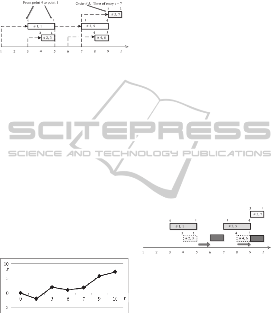
Figure 1: Diagram of orders entry and scheduling.
Let’s calculate the profit of truck# 1 in the Model
#3, where penalties are applied. We will calculate
the profit v at the moments of transition of the truck
from one state to another. Let’s look at the step by
step profit calculation.
Execution of order #1 will require to start at the
moment t=1 from point #1 to point # 4 and will take
2 days till the moment t=3. At the moment t=3 the
profit is P=-q*2=-2. Let’s show the change of the
profit P in real time (Figure 2).
The transportation of cargo from point 4 to the
point 1 will take 2 days, and at t=5 the truck will
arrive at the point 1 with the profit p=-2+(c-q)*2=-
2+2*2=2.
Assume that the truck agent assesses options of
further schedule and execution upon arrival to point
1 at time t=5. Its profit at point 4 is v=2. By this time
order # 3 has been entered at the moment of time #3.
There are two options to execute it:
Order #2 is to be executed with delay;
Order #2 is rejected, idle time cost is
accepted, order #3 from the same point 1 is to be
taken; for order # 2 can be executed with delay
before execution of order #3, no further options
will be taken into consideration. Let’s take a
more precise look at 2 options.
Figure 2: Profit of truck agent depending on time.
Truck needs to reach point 3, moving from point
1 (1 day trip), pick up the order and execute it, going
from point 3 to point 1 (1 day). The increase of
profit is dp=-1*q+(c-q)*1=-1+2=1.
Penalty applied because of delay is -pp*2=-
2*0.6=-1.2. As a result the truck will be at the
moment t=7 at the point 1 with the profit P=2+1-
1.2=1.8. Execution of the order would seem to be
unprofitable, but one should take into consideration
that in case of cancellation of the order the truck
would stay idle for 2 days, and the profit at the
moment t=7 would be P=2-2*0.3=1.4.
That’s why the truck agent is interested in the
execution of order #2 with delay, order #3, t= 7…9
(from point 1 to point 4) - 2 days, profit is
P=1.8+2*(c-q)=1.8+2*2=5.8, and the truck moves to
point 4.
At the moment t=9 new order# 5 comes in at the
point 3 with start time of execution t=9; empty run
to its loading point is 1 day, what puts the order
beyond the 10-days scheduling horizon limit. That’s
why the truck agent rejects the order. There is an
outdated order #4 from point 4 to point 3, its
execution start time should be t=8. The truck agent
assesses profit from possible shift of order by a day.
Execution of the order #4, empty run is not
required, dp=(3-1)*1=2-penalty 0.6=1.4. If this
order were rejected, the truck would stay idle for 1
day till the end of the scheduling horizon and then
dp=-1*0.3=-0.3.. That’s why the truck agent accepts
the order #4.
Outcome: orders #1 and 3 are executed without
delay, order #2 – with allowed delay of 2 days and
order #4 – with allowed delay of 1 day. Order #5 is
rejected (Figure 3).
Total profit in 10 days is P=5.8+1.4=7.2.
Figure 3: Diagram of execution of adaptive schedule by
one truck.
The delayed orders on Figure 3 are shown with
dark grey, when penalties are applied; light grey
marks orders without delay; shifts in schedule are
shown with wide arrows; shifted orders are shown
with dotted borders; rejected order is white (not
visible). White arrows stand for empty runs, light
grey ones – executions of orders with delay; dark
grey ones – executions of orders on time.
As a larger-scale example, task of scheduling of
execution of 100 orders for 10 trucks has been
studied (Figure 4). The Figure 4 shows incoming
orders, where the length of a segment shows a
preferred time of the order execution.
CargoTransportationModelsAnalysisusingMulti-AgentAdaptiveReal-TimeTruckSchedulingSystem
247
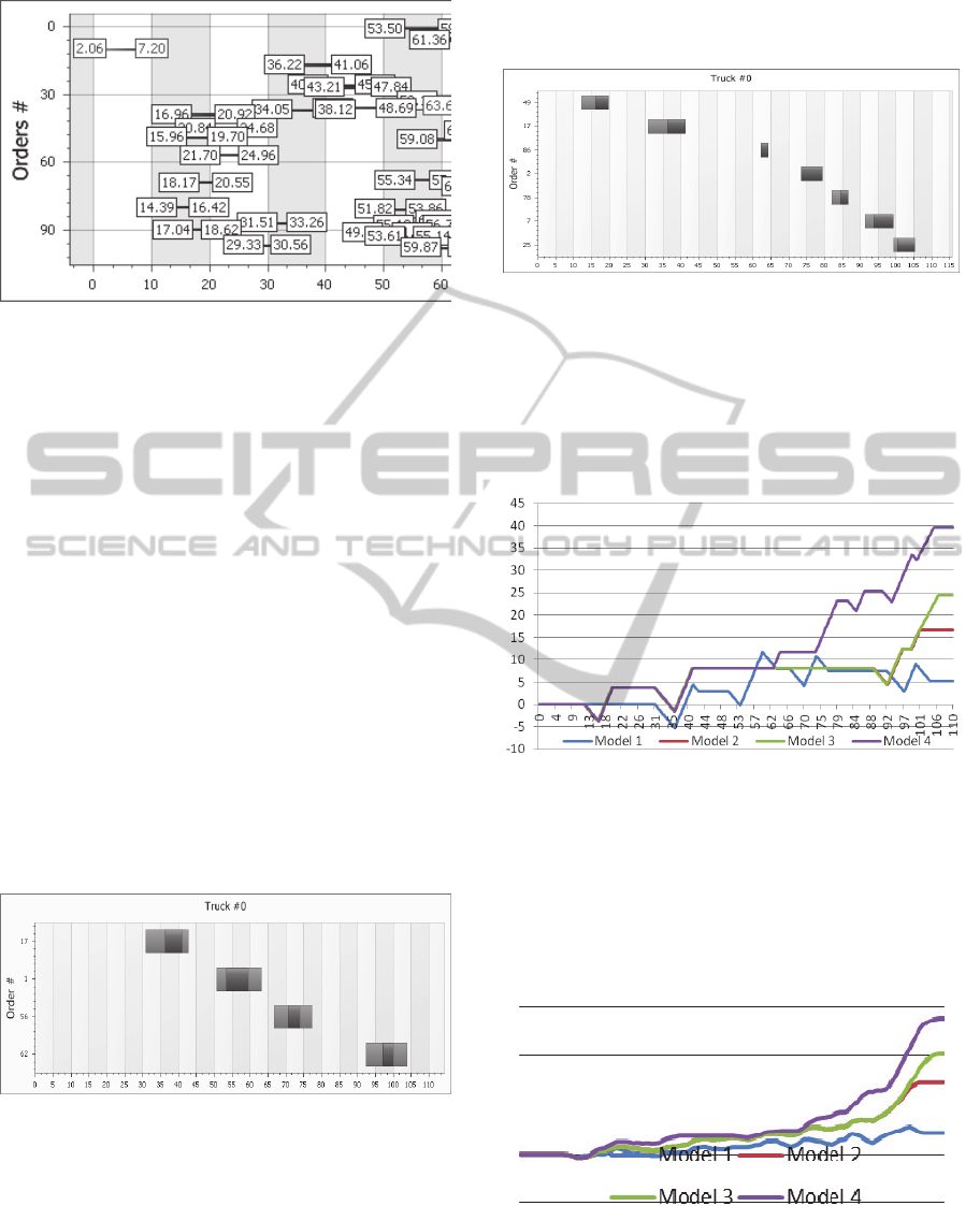
Figure 4: Allocation of input orders in time.
Orders were generated with equal distribution
among cities (points) and by dates. Times of start of
execution are also equally distributed, but all –
within the time of entry and the end of the
scheduling horizon. That’s why the intensity of
orders increases at the end of the time period of
simulation. Trucks are based initially in one point –
base. Orders are distributed equally among 18
points. Distances between points are from 1 to 6.
The scheduling horizon is 100 days.
6 THE RESULTS OF THE
EXPERIMENTS
Trucks schedules were created for orders based on
the 4 used models of transportation. As an example
of the result let’s see the schedule (Gantt chart) of
truck #0 in the Model 1 and Model 4 which are
presented on Figure 5 and Figure 6.
Figure 5: Truck schedule in the Model 1 with returning to
base.
Horizontal axis of Figure 5 and Figure 6 shows
time in days, vertical shows orders numbers. The
executed orders are shown in a dark colour. Brighter
rectangles before an order accord to a trucks running
process in a loading point. Rectangles on the Figure
5 also show a truck that is returning to base point
according the Model 1. Dark rectangle on Figure 6
shows an order that was executed with delay and
penalty.
Figure 6: Truck schedule in the Model 4 with adaptive
reschedule and penalties.
Graphs of dynamic profit per each truck
depending on time was found. Figure 7 shows profit
dynamics for the truck according to Model 1 –Model
4. It accords the truck schedules represented above
by the Gantt chart diagrams.
Figure 7: Dynamics of a profit for the truck depending on
model of transportation.
Straight horizontal segments accord to a truck
stop periods, segments with positive growth show a
profit growth while an order was running, segments
with negative growth show idle run costs of the
truck to the loading point or to the base in the Model
1.
Figure 8: Dynamics of sum of trucks profit depending on
transportation models.
The summary profit for all vehicles in each of
the 4 models of transport is the sum of profits in
ICAART2013-InternationalConferenceonAgentsandArtificialIntelligence
248

each truck. It’s shown in Figure 8.
The designed MAS allows also to study the
profit depending on trucks number for each flow of
orders. For simplicity we don’t consider standing
costs of trucks. For the initial orders schedule
(Figure 4) the trucks schedules and approximate
profit were modeled according to Model 1 – Model
4.
The trucks amount was varied from 0 to 50
(Figure 9).
Figure 9: The dependence of the profit to the used trucks
number in the different transportation models.
Each graph of total profit has two typical
regions. The first region contains an almost linear
increase profits with the number of trucks and the
second is a ’saturation’ region, for which the profit
is almost constant and does not vary with the
number of trucks. That is due to the fact that most of
the new orders have been assigned to the trucks.
Saturation modes differ for the different models.
The lowest profit value is in the Model 1 because
less amount of orders are scheduled and additional
expenses occur after returning to the base. The
Model 3 far exceeds the Model 2 because it uses the
same amount of trucks as in the Model 2 but more
orders are scheduled. But in a satiation mode it gives
almost no benefits vs. the Model 2, because when
the trucks number is high enough there are very few
orders that are executed with delays so The Model 2
and the Model 3 will be almost equal.
The Model 4 is the best one. It gives approximate
20% more profit then the Model 2 and the Model 3.
It allows using less trucks during the plan execution.
The reason is the adaptive re-scheduling of
orders in real time.
7 CONCLUSIONS
The paper studies benefits of multi-agent system for
real time adaptive truck allocation, scheduling and
optimization in long-distance transportations of
cargos.
It was shown that multi-agent technology allows
to create significantly more profitable schedules (up
to 40-60% compared with rigid models) and save a
number of trucks (up to 20%) for the same amount
of orders. The results of the research can be used for
improving management of any type of mobile
resources.
REFERENCES
Leung , Y-T., 2004. Handbook of Scheduling: Algorithms,
Models and Performance Analysis. Chapman & Hall.
London.
Bonabeau, E., Theraulaz, G., 2000. Swarm Smarts. What
computers are learning from them? Scientific
American, vol. 282, no. 3, pp. 54-61.
Wooldridge, M., 2002. An Introduction to Multi-Agent
Systems. JohnWiley & Sons. London, 2
nd
edition.
Vittikh, V., Skobelev, P., 2003. Multi-Agent Models for
Designing Demand-and-Resource Networks in Open
Systems. Automation and Remote Control, vol. 64, no.
1, pp. 162-169.
Skobelev, P., 2010. Bio-Inspired Multi-Agent Technology
for Industrial Applications. Multi-Agent Systems –
Modeling, Control, Programming, Simulations and
Applications. Faisal Alkhateeb, Eslam Al Maghayreh
and Iyad Abu Doush (Ed.). InTech Publishers. Austria.
28 p.
Skobelev, P., 2011. Multi-agent technology for real time
resource allocation, scheduling, optimization and
controlling in industrial applications. In HoloMAS
2011, 5th International Confrence on Industrial
Applications of Holonic and Multi-Agent Systems.
Springer. Berlin. pp. 1-14.
Basra, R., Lü, K., Rzevski, G., Skobelev, P., 2005.
Resolving Scheduling Issues of the London
Underground Using a Multi-Agent System. In Lecture
Notes in Artificial Intelligence (Subseries of Lecture
Notes in Computer Science), 3593. pp. 188-196.
Himoff, J., Rzevski, G., Skobelev, P., 2006. Magenta
Technology: Multi-Agent Logistics i-Scheduler for
Road Transportation. In AAMAS 2006, 5th
International Conference on Autonomous Agents and
Multi Agent Systems. Japan.
Skobelev, P., 2010. Multi-Agent Technologies for
Industrial Applications: Towards 20 years Anniversary
of Samara Scientific School of Multi-Agent Systems.
Mechatronics, Automation, Control, no. 12, pp. 33-
46.
CargoTransportationModelsAnalysisusingMulti-AgentAdaptiveReal-TimeTruckSchedulingSystem
249
