3D Local Binary Pattern for PET Image Classiﬁcation by SVM

Application to Early Alzheimer Disease Diagnosis

Christophe Montagne, Andreas Kodewitz, Vincent Vigneron, Virgile Giraud and Sylvie Lelandais

University of Evry, IBISC Laboratory, 40 Rue du Pelvoux, CE 1455, 91020 Evry Cedex, France

Keywords:

Local Binary Pattern, Feature Extraction, Positron Emission Tomographic images, Alzheimer disease,

Machine Learning.

Abstract:

The early diagnostic of Alzheimer disease by non-invasive technique becomes a priority to improve the life

of patient and his social environment by an adapted medical follow-up. This is a necessity facing the growing

number of affected persons and the cost to our society caused by dementia. Computer based analysis of

Fluorodeoxyglucose PET scans might become a possibility to make early diagnosis more efﬁcient. Temporal

and parietal lobes are the main location of medical ﬁndings. We have clues that in PET images these lobes

contain more information about Alzheimer’s disease. We used a texture operator, the Local Binary Pattern,

to include prior information about the localization of changes in the human brain. We use a Support Vector

machine (SVM) to classify Alzheimer’s disease versus normal control group and to get better classiﬁcation

rates focusing on parietal and temporal lobes.

1 INTRODUCTION

The number of people affected by the Alzheimer Dis-

ease (AD) is growing. In 2010, this dementia af-

fected 35.6 million people (Wimo and Prince, 2010).

This disease affects patient himself and his social

environment. The detection of the early states of

Alzheimer disease allows to begin some treatments

for the patient and slow down the progress of the dis-

order (Salmon, 2008). Most of works focused on tem-

poral lobes, few of them on parietal lobes (Kodewitz

et al., 2011). Some works on the SPECT-scans (Sin-

gle Photon Emission Computed Tomography) are due

to Ramìrez with a computer-aided diagnosis based

on a selection of image parameters (ﬁrst and second

order statistics) and Support Vector Machine (SVM)

(Ramìrez et al., 2009). Others methods with PET-

scans (Positron Emission Tomography) are based on

covariance analysis of voxels to classify AD versus

Normal Control (NC) (Scarmeas et al., 2004). The

main idea of this work is that we can automatically

analyse the PET scans to detect AD patient versus

NC patient using textural features. This classiﬁca-

tion can help doctors to make their early diagnostic

and try to localize some brain areas where Alzheimer

Disease is growing. In our study, we use 3D-scans

extracted from the ADNI database (Alzheimer’s Dis-

ease Neuroimaging Initiative) and we propose to use

a textural operator which is the Local Binary Pattern

(LBP) (Pietikäinen and Ojala, 2000) extended to the

3D. Then this new feature was studied by an ANaly-

sis Of VAriance (ANOVA). The analysis highlighted

a link between LBP patterns and the type of patient

or some brain areas. Based on this new feature, we

train a machine learning algorithm SVM to classify

AD versus NC PET-scans. For this step, in a ﬁrst time

we use as Region Of Interest (ROI) parietal and tem-

poral lobes, and then, in a second time full PET-scans

are considered.

In the ﬁrst section we describe the materials used

in this study. Secondly we introduce the 3D Local

Binary Pattern that we developed. Then we explain

the ANOVA method and the obtained results. Finally

after a short presentation of SVM, we discuss on the

results of the classiﬁcation using the LBP caracteris-

tics and we conclude.

2 MATERIALS

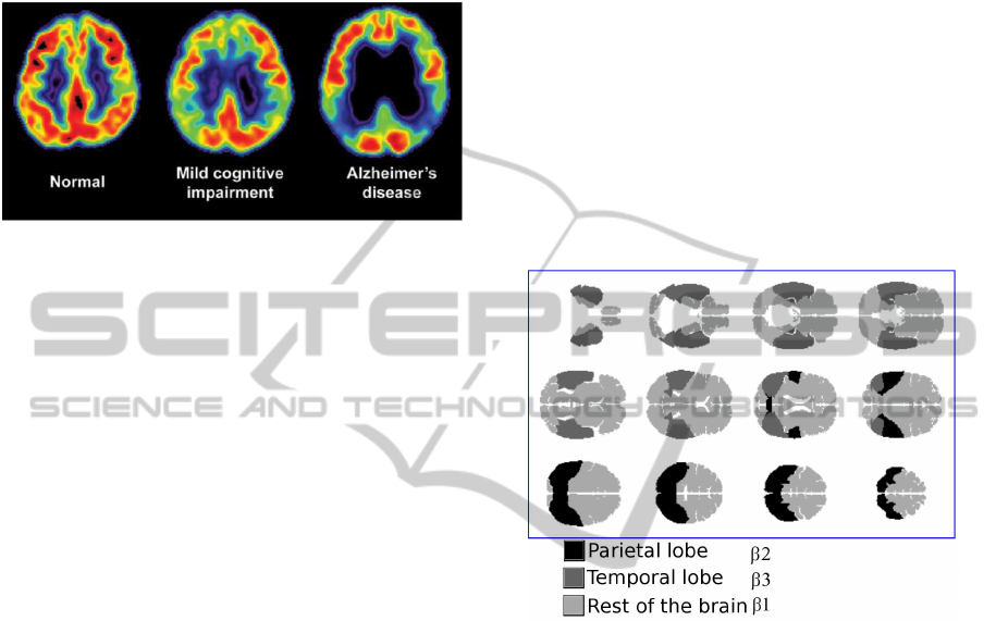
In this study, PET-scan provides three-dimensional

functional imaging data that measures the metabolism

in the brain which are acquired by a non-invasive

method, Figure 1 shows how the AD reduces the

metabolism in the brain. This scan is obtained by 18F-

145

Montagne C., Kodewitz A., Vigneron V., Giraud V. and Lelandais S..

3D Local Binary Pattern for PET Image Classiﬁcation by SVM - Application to Early Alzheimer Disease Diagnosis.

DOI: 10.5220/0004226201450150

In Proceedings of the International Conference on Bio-inspired Systems and Signal Processing (BIOSIGNALS-2013), pages 145-150

ISBN: 978-989-8565-36-5

 2013 SCITEPRESS (Science and Technology Publications, Lda.)

ﬂuorodesoxyglucose (in short 18F-FDG) injection to

a patient. This radioactive isotope allows to capture

the distribution of brain activity. With this technique,

we can detect the ﬁrst abnormalities before structural

alteration (Bennys et al., 2001).

Figure 1: PET scans of AD, MCI and NC patient.

2.1 ADNI Database

The American Alzheimer’s Disease Neuroimaging

Initiative (ADNI, http:// www.loni.ucla.edu/ ADNI/)

collects data of patients affected by AD, mild cog-

nitive impairment (MCI) and normal control group

(NC). This includes diagnosis based on mental state

exams (e.g. mini mental state exam (MMSE)),

biomarkers, MRI and PET scans. In this database we

chose PET scans with 18F-FDG tracer from AD and

NC patients. Each image contains 91×109 ×91 vox-

els after normalization (the PET-scans have initially

different sizes). For our purpose we extracted 166 3D-

scans (one 3D-scan for one patient) which are sorted

in 82 AD and 84 NC. Moreover, the AD scans are

taken early in the disease to simulate a situation of

early diagnosis.

2.2 Brain Atlas

Today, the deﬁnite diagnosis of AD is based on the

post-mortem observation of intracellular neuroﬁbril-

lary tangles (NTF): β-amyloid deposition in the form

of extracellular senile plaques and blood vessel de-

posits, synapse dysfunction and loss. NTF deposition

originates in the medial temporal lobes and then be-

gins to cluster in the adjacent inferior temporal and

posterior cingulate cortex in mild AD, and ﬁnally

spreads to the parieto-temporal and prefrontal associ-

ation cortices. Medical doctors use this information in

their analysis of PET scans. They search for abnormal

variations in the brain metabolism and do their diag-

nosis based on the location of these abnormalities. In

order to emulate this method, we decide to use a brain

atlas which gives us a brain model. With the

Matlab

toolbox WFU PickAtlas (Maldjian et al., 2003), using

the Talairach daemon by Lancaster et al. (Lancaster

et al., 2000), it is even possible for nonspecialists to

select a volume of interest in the brain by knowing

the name of a certain area, e.g. the name of the lobe,

and create an indexed mask for this volume of inter-

est. We used these prerequisites to create a simpliﬁed

map which distinguishes only three zones: temporal

lobes, parietal lobes and the rest of the brain (see ﬁg-

ure 2). Each voxel of a PET-scan matches with a voxel

of this atlas because our atlas size is the same as our

normalised brain PET-scans. So we have a unique

model of brain for all individuals. Parietal and tem-

poral areas are considered identical from one brain

to another and adopt a location and volume average.

Parietal lobes contain 26850 voxels, temporal lobes

contains 33103 voxels and rest of the brain contain

119907 voxels in each PET-scan.

Figure 2: Brain atlas.

3 LOCAL BINARY PATTERN

3.1 2D Local Binary Pattern

LBP was proposed by Pietikäinen et Ojala in the 90’s

(Pietikäinen and Ojala, 2000). The idea is to give a

pattern code to each pixel. Gray level of the central

pixel g

is compared to gray level of each neighboring

pixel g

. Then by thresholding, a value of 0 or 1 is

associated to each neighboring pixel.

LBP

P,R

P−1

∑

i=0

s(g

− g

, with s(x) =

(

1 if x ≥ 0

0 else.

(1)

where P is the number of neighbor pixels separated

from R pixel(s) to the central pixel c. Figure 3 illus-

trates this feature.

BIOSIGNALS2013-InternationalConferenceonBio-inspiredSystemsandSignalProcessing

146

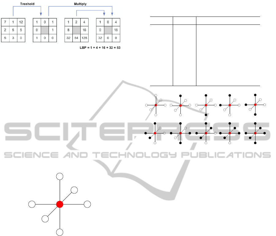
Figure 3: Example of 2D-LBP with P = 8 and R = 1.

3.2 3D Local Binary Pattern

The main idea of this work is an adaptation of the LBP

to capture the 3D structure of texture. We need LBP

patterns which have a rotation invariance and qualify

the AD PET-scans. Some works have been performed

on the extend of the Local Binary Pattern method for

characterisation of 3D textures by L. Paulhac (Paul-

hac et al., 2008). His vision of 3D-LBP consists on

a superposition of circles that represent a spherical

neighborhood. Each circle can be encoded like a 2D-

LBP. Our proposition consists to select 6 nearest vox-

els and to order them for encoding pattern (see ﬁgure

4).

Figure 4: 3D-LBP with 6 neighbors LBP

6,1

By this way, we have 2

= 64 possible patterns

that we merge in 10 groups according to geometrical

similarities (see ﬁgure 5). Each group is ﬁlled with

patterns which have the same numbers of neighbor

voxels with a gray level higher than the central voxel

c. The idea was to keep a rotation invariance in each

group. Table 1 deﬁnes these groups with:

card(c) =

P−1

∑

i=0

s(g

− g

) (2)

where P = 6 is the number of voxels in neighborhood

and R = 1 or R = 2 the distance between the central

voxel and its neighbors. We use two values of R to

capture micro and macro-structure of the texture with

our 3D-LBP. In equation 2, card(c) gives the number

of neighbors with an higher gray level than the central

voxel.

Table 1: Deﬁnition of the 10 groups of patterns rotationally

invariant.

LBP

P,R

card(c) condition

1 0

2 1

3 2 opposite voxels

4 2 bend voxels

5 3 voxels on the same plane

6 3 voxels on different planes

7 4 voxels on the same plane

8 4 voxels on different planes

9 5

10 6

1(1) 3(3)2(6)

9(6)8(12) 10(1)

6(8)

7(3)

4(12) 5(12)

Figure 5: Merging of 2

= 64 patterns in 10 groups. The

integer in brackets indicates the number of different patterns

for each group.

In our experimental protocol, the count of these

patterns in ROI of PET-scans or in full PET-scans will

be the input variable of our machine learning algo-

rithm.

3.3 ANOVA

The 3D-LBP features may be an important character

for the classiﬁcation of Alzheimer PET-scan. We per-

form an analysis of variance to ﬁnd the link between

a variable of interest (the count of 3D-LBP features)

and some response variables (type of patient, brain

area, type of pattern) which are also called factors and

its relevance.

Suppose that the variable to explain Y follows a

normal distribution in each population. y

i j

was a re-

alization of Y ∼ N (µ

,σ). There are two hypothe-

sis: H

-Null hypothesis, every data follows a normal

distribution; H

-At least one sample follows an other

normal distribution.

There are 3 factors:

• α

: type of patient (AD/NC),

• β

: brain area (temporal lobe β

, parietal lobe β

rest of brain β

, full brain β

) (see ﬁgure 2),

• γ

: type of pattern (1 .. . 10) (see ﬁgure 5).

We search the inﬂuence of a factor set (α

, β

, γ

)

on the variable of interest Y . This method can be ap-

3DLocalBinaryPatternforPETImageClassificationbySVM-ApplicationtoEarlyAlzheimerDiseaseDiagnosis

147

plied on each factor or on all together. For example,

Eqs. 3 and 4 show a case with a single factor.

= µ + m

+ ε

(3)

where µ is an offset, m

the theoretical mean of

the sample i and ε

are Gaussian i.i.d error terms

(N (0,σ

)).



















1 0 0

0 1 0



























(4)

where m is the theoretical mean of the sample. This

equation shows the variance decomposition:

∑

i=1

∑

k=1

− m)

∑

i=1

− m)

∑

i=1

∑

k=1

(5)

= SC

+ S

and m are estimated by: ¯y

∑

i=1

and ¯y =

∑

i=1

∑

k=1

. Under H

, we have:

∼ χ

n−1

∼ χ

3−1

∼ χ

n−3

(6)

and:

T =

/(3 − 1)

/(n − 3)

∼ F

p−1,n−p

. (7)

Under H

, the statistics T follows a Fisher distri-

bution with (3 − 1,n − 3) degrees of freedom. The

critical value is T > F

p−1,n−p,1−α

, where α settles the

conﬁdence level with which one can reject the hy-

pothesis H

(by convention often chosen to be 95%).

Table 2 exposes a part of the results. The p-value

of each group of pattern on each area of brain is dis-

played.

The p-value is the probability of obtaining a test

statistic at least as extreme as the one that was actu-

ally observed, assuming that the H

hypothesis is true.

The lower is the p-value, the higher is the probabil-

ity of H

to be true. We choose a p-value threshold

to 0.005: we accept H

is true with 99.5% or more

(bold p-values in the table). We can see p-values cor-

responding to the full brain (β

) or rest of the brain

(β

) are higher than our threshold: the count of the

3D-LBP patterns is not informative in these areas. In

the parietal and temporal lobes (β

, β

), we notice the

Table 2: p-values for the different brain areas.

LBP Group

number

Pr(> F)

1 2.13e-1 1.42e-1 5.83e-5 2.63e-2

2 5.47e-1 3.14e-1 1.66e-5 1.86e-4

3 2.71e-1 6.38e-1 3.14e-4 2.51e-7

4 7.89e-1 1.60e-1 1.76e-3 1.07e-2

5 9.77e-1 2.24e-1 8.60e-5 4.69e-3

6 7.61e-1 4.20e-1 1.56e-3 5.72e-3

7 9.22e-1 3.38e-1 7.40e-3 1.39e-1

8 7.62e-1 4.13e-1 2.50e-3 1.79e-3

9 6.00e-1 2.12e-2 3.22e-3 3.69e-1

10 3.49e-1 2.54e-2 1.86e-1 6.43e-2

power of some LBP patterns for discriminating the

type of patient α

These observations allow to use machine learning

to create a classiﬁer with the 3D LBP features ex-

tracted from the PET-scan.

4 CLASSIFICATION BY

SUPPORT VECTORS MACHINE

The SVM was introduced by Vapnik (Vapnik, 1998).

We used a description of the SVM which is based on

Schölkopf and Smola (Schölkopf and Smola, 2002)

works. Consider a training data set consisting of two

separable classes in a n-dimensional feature space.

This means each class forms its own cluster and those

clusters do not intersect. From this follows that there

exists at least one hyperplane able to separate the two

classes with one class on each side of the hyperplane.

We use a Gaussian kernel in SVM, γ ≥

0, k(x, x

) = e

(−||x−x

/γ

)

. In ﬁgure 6 we can see

the contour plot of the error landscape resulting from

a grid search on hyperparameter cost C and gamma γ.

C is a cost constant for the Lagrangian. This grid is

obtained with the function tune in R. The red circle

shows the area with the best parameters.

PET-scans used in this study come from the ADNI

database. Each scan contains 91 × 109 × 91 voxels.

We selected 82 patients from AD group and 84 from

NC group (one patient = one PET-scan). We try to

classify AD versus NC. Each voxel in the image is

encoded by LBP

6,1

and LBP

6,2

. We have 10, 20 or

30 input variables if we use 1, 2 or 3 areas of brain

(parietal β

, temporal β

, rest of the brain β

) in the

classiﬁer. With full brain (β

) we have 10 variables.

And when we use the LBP

6,1

and LBP

6,2

, the number

of variables is doubled.

These variables constitute our input vector for

SVM. In table 3 we see the classiﬁcation rate for the

3 brain areas or for parietal and temporal lobes. Other

BIOSIGNALS2013-InternationalConferenceonBio-inspiredSystemsandSignalProcessing

148

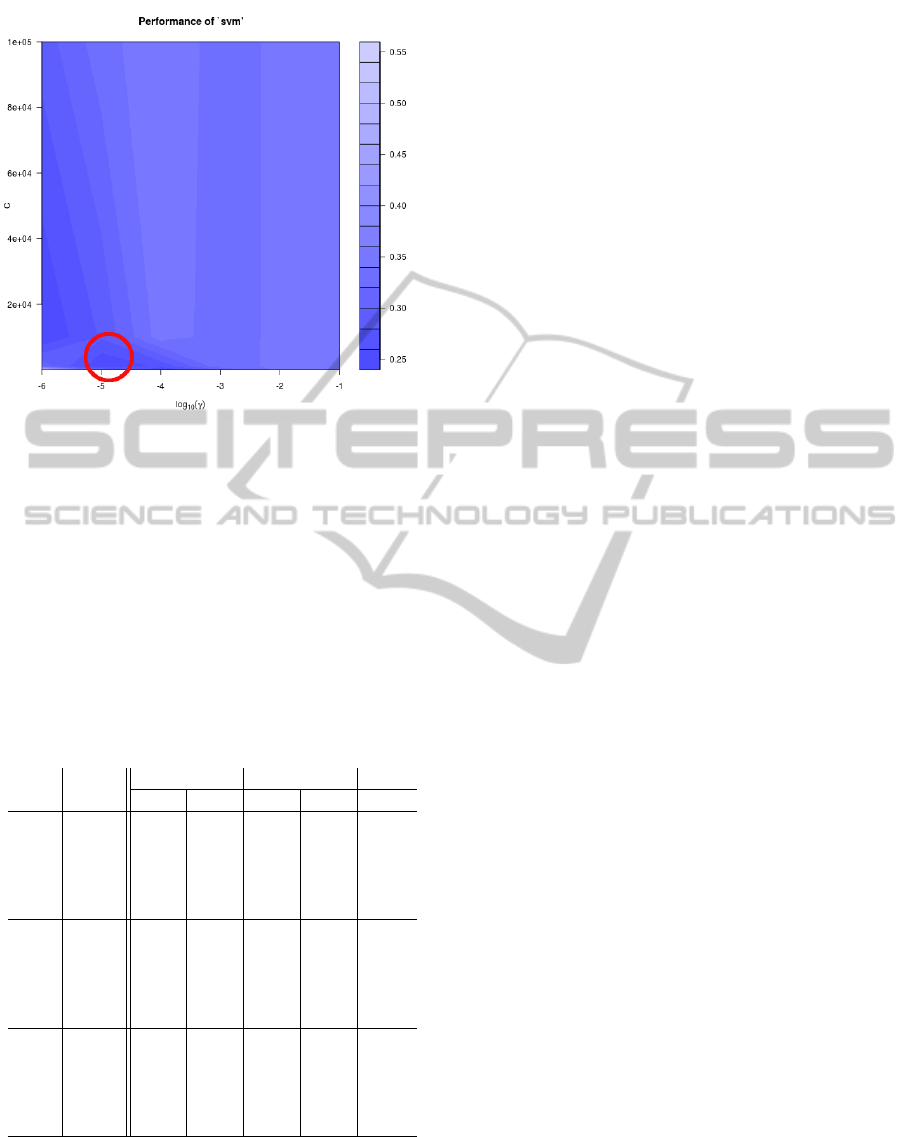
Figure 6: Visualisation of the tuning parameters C and γ.

results with only one brain area (β

, β

or β

) or full

brain (β

) don’t appear in this table because of lower

results. The cross validation consists in a number of

runs equal to size of the base of a SVM. For each run

we divide the main database with a part used for train-

ing and the other for testing. The mean of all these

runs give us the rate of cross validation.

Table 3: Precision, recall and cross validation (CV) for

SVM classiﬁcation - ¬: LBP

6,1

, : LBP

6,2

. β

1,2,3

is put

for the use of all brain areas; β

2,3

is for temporal and pari-

etal lobes.

LBP Brain Precision Recall

type areas AD NC AD NC CV

68% 70% 70% 68% 60%

67% 70% 70% 67% 68%

¬ β

75% 71% 67% 79% 64%

1,2,3

89% 81% 79% 90% 75%

2,3

85% 79% 76% 86% 66%

64% 67% 68% 63% 56%

73% 70% 66% 76% 70%

 β

65% 71% 68% 76% 66%

1,2,3

87% 79% 76% 89% 75%

2,3

82% 82% 81% 83% 68%

74% 77% 77% 74% 63%

¬ β

74% 70% 67% 77% 69%

& β

77% 72% 67% 81% 67%

 β

1,2,3

87% 79% 76% 89% 77%

2,3

82% 82% 81% 83% 69%

Table 3 shows results obtained with different vari-

ables of LBP

6,1

and LBP

6,2

. We can notice that all the

results are very close together. But when we use the

3 brain areas, the SVM classiﬁer reaches better rates

than just using parietal and temporal lobes. The best

CV rate is 77% with LBP

6,1

&LBP

6,2

. We can assume

that this value is relatively low because the scans cor-

respond to the beginning of the disease when the di-

agnosis is more difﬁcult than for a patient severely

affected.

5 CONCLUSIONS

We propose a new method to identify patients af-

fected by the Alzheimer Disease from their PET-scan.

With the ANOVA we have shown LBP are impor-

tant features to class AD versus NC PET-scans. Then

we train and test a classiﬁer to create an automatic

computer-aided diagnosis for the Alzheimer Disease

using the LBP caracteristics extracted from the PET-

scan. We reach to a score of 77% by using SVM

method with LBP

6,1

and LBP

6,2

patterns.

Currently we improve this work by slicing in

small cubes, in each of these block we count the LBP

patterns. Then these counts are used as variables for a

Random Forest classiﬁcation. RF is adapted to com-

pute and to have a good classiﬁcation rate with this

high number of features.

An other way to improve the results can be to de-

velop some new LBP types to capture more accurately

the texture of brain in the PET-scans. We can notice

that some regions that are outside temporal and pari-

etal lobe contain also a certain amount of discrim-

inating information which is captured with our ap-

proach. In this case we can extend the analysed brain

areas to ﬁnd other ROI. A brain mapping of each PET-

scan can be used to deﬁne more cleverly position of

the temporal and parietal lobes, or some other sub-

parts. The idea is to customize an atlas for each pa-

tient rather than our standard atlas for all the database.

This way is already used on IRM-scans. With this, we

have to segment brain to ﬁnd the edges of the differ-

ent areas. In the same way, merge IRM and PET data

will be an interesting search.

ACKNOWLEDGEMENTS

Data used in the preparation of this arti-

cle were obtained from the Alzheimer’s Dis-

ease Neuroimaging Initiative (ADNI) database

(www.loni.ucla.edu/ADNI). As such, the investi-

gators within the ADNI contributed to the design

and implementation of ADNI and/or provided data

but did not participate in analysis or writing of

this report. ADNI investigators include (complete

listing available at http://www.loni.ucla.edu/ADNI/

Collaboration/ADNI_Manuscript_Citations.pdf).

3DLocalBinaryPatternforPETImageClassificationbySVM-ApplicationtoEarlyAlzheimerDiseaseDiagnosis

149

REFERENCES

Bennys, K., Rondouin, G., Vergnes, C., and Touchon,

J. (2001). Diagnostic value of quantitative EEG

in alzheimer’s disease. Clinical Neurophysiology,

31(3):153–160.

Kodewitz, A., V., V., Montagne, C., and Lelandais, S.

(2011). Where to search for alzheimer’s disease re-

lated changes in pet scans? RITS, Rennes, France.

Lancaster, L., Woldorff, M. G., and Parsons, L. M. (2000).

Automated talairach atlas labels for functional brain

mapping. Human Brain Mapping, 10:120–131.

Maldjian, J. A., Laurienti, P. J., Burdette, J. H., and

Kraft, R. A. (2003). An automated method for neu-

roanatomic and cytoarchitectonic atlas-based interro-

gation of fmri data sets. NeuroImage, 19:1233–1239.

Paulhac, L., Makris, P., and Ramel, J. (2008). Compari-

son between 2d and 3d local binary pattern methods

for characterisation of three-dimensional textures. In

Series, B., editor, Lecture Notes in Computer Science,

volume 5112/2008, pages 670–679, Pòvoa de Varzim,

Portugal. ICIAR.

Pietikäinen, M. and Ojala, T. (2000). rotation-invariant tex-

ture classiﬁcation using feature distributions. Pattern

Recognition, 33:43–52.

Ramìrez, J., Gòrriz, J., and et al., D. S.-G. (2009).

Computer-aided diagnosis of alzheimer’s type demen-

tia combining support vector machines and discrimi-

nant set of features. Information Sciences.

Salmon, E. (2008). Différentes facettes de la maladie de

type azheimer. Rev Med Liege, 63(5-6):299–302.

Scarmeas, N., Habeck, C. G., and et al., E. Z. (2004). Co-

variance pet patterns in early alzheimer’s disease and

subjects with cognitive impairment but no dementia:

utility in group discrimination and correlations with

functional performance. NeuroImage, 23(1):35 – 45.

Schölkopf, B. and Smola, A. (2002). Learning with Ker-

nels - Support Vector Machines, Regularization, and

Beyond. The MIT Press.

Vapnik, V. (1998). Statistical learning theory. Wiley.

Wimo, A. and Prince, M. (2010). World alzheimer report

2010. http://www.alz.co.uk/research/world-report.

BIOSIGNALS2013-InternationalConferenceonBio-inspiredSystemsandSignalProcessing

150