
Unsupervised and Transfer Learning under Uncertainty
From Object Detections to Scene Categorization
Gr
´
egoire Mesnil
1,2
, Salah Rifai
1
, Antoine Bordes
3
,
Xavier Glorot
1
, Yoshua Bengio
1
and Pascal Vincent
1
1
LISA, Universit
´
e de Montr
´
eal, Qu
´
ebec, Canada
2
LITIS, Universit
´
e de Rouen, Rouen, France
3
CNRS - Heudiasyc UMR 7253, Universit
´
e de Technologie de Compi
`
egne, Compi
`
egne, France
Keywords:
Unsupervised Learning, Transfer Learning, Deep Learning, Scene Categorization, Object Detection.
Abstract:
Classifying scenes (e.g. into “street”, “home” or “leisure”) is an important but complicated task nowadays,
because images come with variability, ambiguity, and a wide range of illumination or scale conditions. Stan-
dard approaches build an intermediate representation of the global image and learn classifiers on it. Recently,
it has been proposed to depict an image as an aggregation of its contained objects:the representation on which
classifiers are trained is composed of many heterogeneous feature vectors derived from various object de-
tectors. In this paper, we propose to study different approaches to efficiently combine the data extracted by
these detectors. We use the features provided by Object-Bank (Li-Jia Li and Fei-Fei, 2010a) (177 different
object detectors producing 252 attributes each), and show on several benchmarks for scene categorization that
careful combinations, taking into account the structure of the data, allows to greatly improve over original re-
sults (from +5% to +11%) while drastically reducing the dimensionality of the representation by 97% (from
44,604 to 1,000).
1 INTRODUCTION
Automatic scene categorization is crucial for many
applications such as content-based image indexing
(Smeulders et al., 2000) or image understanding. This
is defined as the task of assigning images to pre-
defined categories ( “office”, “sailing”,“mountain”,
etc.). Classifying scene is complicated because of the
large variability of quality, subject and conditions of
natural images which lead to many ambiguities w.r.t.
the corresponding scene label.
Standard methods build an intermediate represen-
tation before classifying scenes by considering the
image as a whole (Torralba, 2003; Vogel and Schiele,
2004; Fei-Fei and Perona, 2005; Oliva and Torralba,
2006). In particular, many such approaches rely on
power spectral information, such as magnitude of spa-
tial frequencies (Oliva and Torralba, 2006) or local
texture descriptors (Fei-Fei and Perona, 2005). They
have shown to perform well in cases where there are
large numbers of scene categories.
Another line of work conveys promising potential
in scene categorization. First applied to object recog-
nition (Farhadi et al., 2009), attribute-based methods
have now proved to be effective for dealing with com-
plex scenes. These models define high-level represen-
tations by combining semantic lower-level elements,
e.g., detection of object parts. A precursor of this ten-
dency for scenes was an adaptation of pLSA (Hof-
mann, 2001) to deal with “visual words” proposed by
(Bosch et al., 2006). An extension of this idea con-
sists in modeling an image based on its content i.e. its
objects (Espinace et al., 2010; Li-Jia Li and Fei-Fei,
2010a). Hence, the Object-Bank (OB) project (Li-
Jia Li and Fei-Fei, 2010b) aims at building high-
dimensional over-complete representations of scenes
(of dimension 44,604) by combining the outputs of
many object detectors (177) taken at various poses,
scales and positions in the original image (leading
to 252 attributes per detector). Experimental results
indicate that this approach is effective since simple
classifiers such as Support Vector Machines trained
on their representations achieve state-of-the-art per-
formance. However, this approach suffers from two
flaws: (1) curse of dimensionality (very large number
of features) and (2) individual object detectors have
a poor precision (30% at most). To solve (1), the
original paper proposes to use structured norms and
345
Mesnil G., Rifai S., Bordes A., Glorot X., Bengio Y. and Vincent P. (2013).
Unsupervised and Transfer Learning under Uncertainty - From Object Detections to Scene Categorization.
In Proceedings of the 2nd International Conference on Pattern Recognition Applications and Methods, pages 345-354
DOI: 10.5220/0004227803450354
Copyright
c
SciTePress

group sparsity to make best use of the large input. Our
work studies new ways to combine the very rich in-
formation provided by these multiple detectors, deal-
ing with the uncertainty of the detections. A method
designed to select and combine the most informative
attributes would be able to carefully manage redun-
dancy, noise and structure in the data, leading to better
scene categorization performance.
Hence, in the following, we propose a sequential
2-steps strategy for combining the feature representa-
tions provided by the OB object detectors on which
the linear SVM classifier is destined to be trained for
categorizing scenes. The first step adapts Principal
Components Analysis (PCA) to this particular set-
ting: we show that it is crucial to take into account
the structure of the data in order for PCA to perform
well. The second one is based on Deep Learning.
Deep Learning has emerged recently (see (Bengio,
2009) for a review) and is based on neural network
algorithms able to discover data representations in
an unsupervised fashion (Hinton et al., 2006; Bengio
et al., 2007; Ranzato et al., 2007; Kavukcuoglu et al.,
2009; Jarrett et al., 2009). We propose to use this
ability to combine multiple detector features. Hence,
we present a model trained using Contractive Auto-
Encoders (Rifai et al., 2011b; Rifai et al., 2011a),
which have already proved to be efficient on many
image tasks and has contributed to winning a transfer
learning challenge (Mesnil et al., 2012).
We validate the quality of our models in an ex-
tensive set of experiments in which several setups of
the sequential feature extraction process are evalu-
ated on benchmarks for scene classification (Lazeb-
nik et al., 2006; Li and Fei-Fei, 2007; Quattoni and
Torralba, 2009; Xiao et al., 2010). We show that
our best results substantially outperform the original
methods developed on top of OB features, while pro-
ducing representations of much lower dimension. The
performance gap is usually large, indicating that ad-
vanced combinations are highly beneficial. We show
that our method based on dimensionality reduction
followed by deep learning offers a flexibility which
makes it able to benefit from semi-supervised and
transfer learning.
2 SCENE CATEGORIZATION
WITH OBJECT-BANK
Let us begin by introducing the approach of the OB
project (Li-Jia Li and Fei-Fei, 2010a). First, the
177 most useful (or frequent) objects were selected
from popular image datasets such as LabelMe (Rus-
sell et al., 2008), ImageNet (Deng et al., 2009) and
Flickr. For each of these 177 objects, a specific de-
tector, existing in the literature (Felzenszwalb et al.,
2008; Hoiem et al., 2005), was trained. Every de-
tector is composed of 2 root filters depending on the
pose, each one coming with its own deformable pat-
tern of parts, e.g., there is one root filter for the front-
view of a bike and one for the side-view. These
354 = 177× 2 part-based filters (each composed by a
root and its parts) are used to produce features of nat-
ural images. For a given image, a filter is convolved
at 6 different scales. At each scale, the max-response
among 21 = 1 + 4+16 positions (whole image, quad-
rants, quadrants within each quadrant) is kept, pro-
ducing a response map of dimension 126 = 6 × 21.
All 2 × 177 maps are finally concatenated to pro-
duce an over-complete representation x ∈ R
44,604
of
the original image.
In the original OB paper (Li-Jia Li and Fei-Fei,
2010a), classifiers for scene categorization are learned
directly on these feature vectors of dimension 44, 604.
More precisely, C classifiers (Linear SVM or Logis-
tic Regression) are trained in a 1-versus-all setting in
order to predict the correct scene category y
category
(x)
among C different categories. Various strategies using
structured sparsity with combinations of `
1
/`
2
norms
have been proposed to handle the very large input.
3 UNSUPERVISED FEATURE
LEARNING
The approach of OB for the task of scene categoriza-
tion, based on specific object detectors, is appealing
since it works well in practice. This suggests that a
scene is better recognized by first identifying basic
objects and then exploiting the underlying semantics
in the dependencies between the corresponding detec-
tors.
However, it appears that none of the individual ob-
ject detectors reaches a recognition precision of more
than 30%. Hence, one may question whether the
ideal view that inspired this approach (and expressed
above) is indeed the reason of OB’s success. Alter-
natively, one may hypothesize that the 44,604 OB
features are more useful for scene categorization be-
cause they represent high level statistical properties
of images than because they precisely report the ab-
sence/presence of objects − see Figure 1. OB tried
structured sparsity to handle this feature selection but
there may be other ways – simpler or not.
This paper investigates several ways of learning
higher-level features on top of the high dimensional
representation provided by OB, expecting that cap-
turing further structure may improve categorization
ICPRAM2013-InternationalConferenceonPatternRecognitionApplicationsandMethods
346
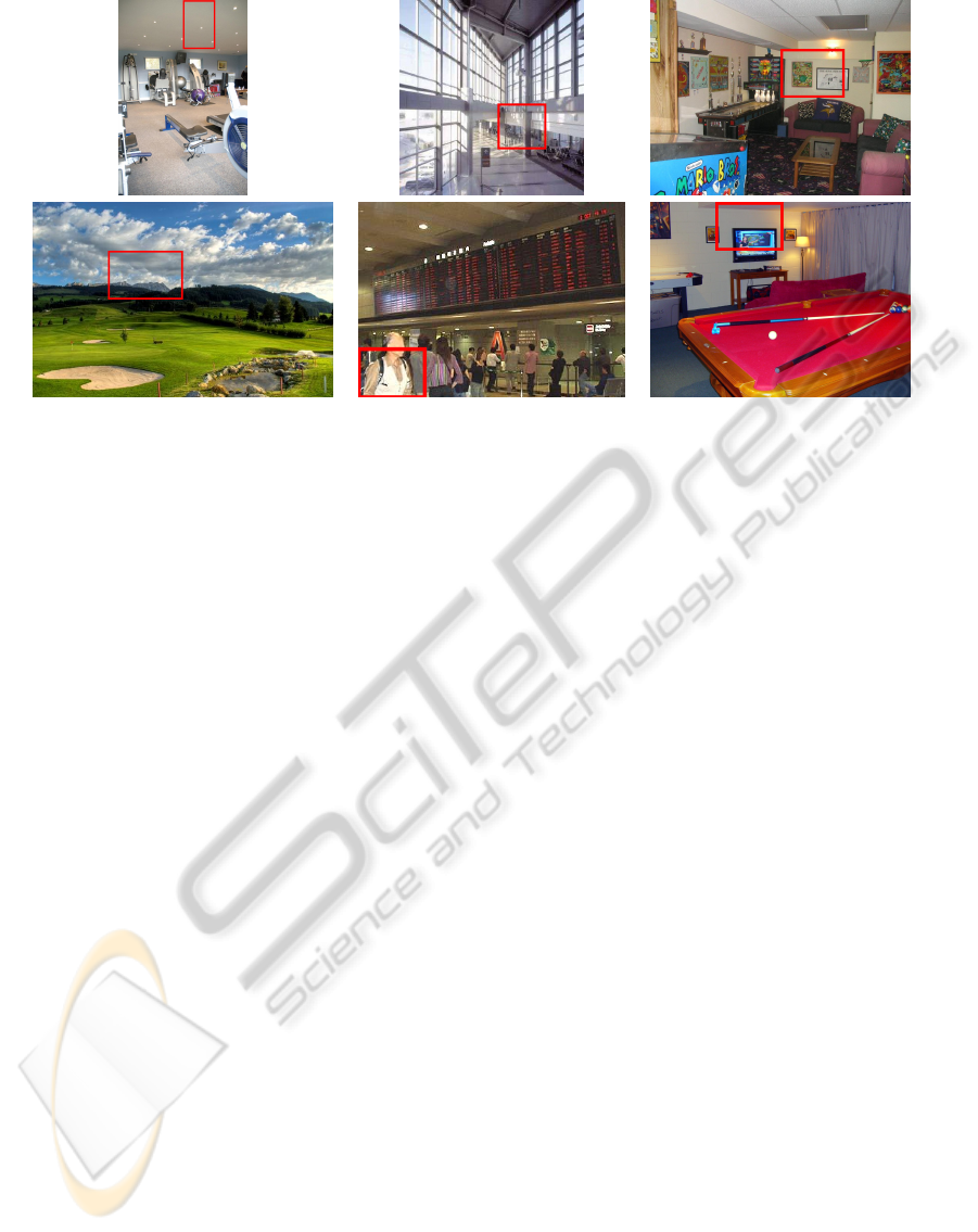
Figure 1: Left: Cloud Middle: Man Right: Television. Top: False Detections Bottom: True Detections. Images from
SUN (Xiao et al., 2010) for which we compute the OB representation and display the bounding box around the average
position of various objects detectors. For instance, the television detector can be viewed either as a television detector or a
rectangle shape detector i.e. high-order statistical properties of the image.
performance. Our approach employs unsupervised
feature learning/extraction algorithms, i.e. generic
feature extraction methods which were not devel-
oped specifically for images. We will consider both
standard Principal Component Analysis and Contrac-
tive Auto-Encoders (Rifai et al., 2011b; Rifai et al.,
2011a). The latter is a recent machine learning
method which has proved to be a robust feature ex-
traction tool.
3.1 Principal Component Analysis
Principal Component Analysis (PCA) (Pearson,
1901; Hotelling, 1933) is the most prevalent tech-
nique for linear dimensionality reduction. A PCA
with k components finds the k orthonormal directions
of projection in input space that retain most of the
variance of the training data. These correspond to
the eigenvectors associated with the leading eigenval-
ues of the training data’s covariance matrix. Principal
components are ordered, so that the first corresponds
to the direction along which the data varies the most
(largest eigenvalue), etc. . .
Since we will consider an auto-encoder variant
(presented next), we should mention here a well-
known result: a linear auto-encoder with k hidden
units, trained to minimize squared reconstruction er-
ror, will learn projection directions that span the same
subspace as a k component PCA (Baldi and Hornik,
1989). However the regularized non-linear auto-
encoder variant that we consider below is capable
of extracting qualitatively different, and usually more
useful, nonlinear features.
3.2 Contractive Auto-encoders
Contractive Auto-Encoders (CAEs) (Rifai et al.,
2011b; Rifai et al., 2011a) are among the latest de-
velopments in a line of machine learning research on
nonlinear feature learning methods, that started with
the success of Restricted Boltzmann Machines (Hin-
ton et al., 2006) for pre-training deep networks, and
was followed by other variants of auto-encoders such
as sparse (Ranzato et al., 2007; Kavukcuoglu et al.,
2009; Goodfellow et al., 2009) and denoising auto-
encoders (Vincent et al., 2008). It was selected here
mainly due to its practical ease of use and recent em-
pirical successes.
Unlike PCA that decomposes the input space
into leading global directions of variations, the CAE
learns features that capture local directions of varia-
tion (in some regions of input space). This is achieved
by penalizing the norm of the Jacobian of a latent rep-
resentation h(x) with respect to its input x at train-
ing samples. Rifai et al. (Rifai et al., 2011b) show
that the resulting features provide a local coordinate
system for a low dimensional manifold of the input
space. This corresponds to an atlas of charts, each
corresponding to a different region in input space, as-
sociated with a different set of active latent features.
One can think about this as being similar to a mixture
of PCAs, each computed on a different set of training
samples that were grouped together using a similarity
criterion (and corresponding to a different input re-
gion), but without using an independent parametriza-
tion for each component of the mixture, i.e., allow-
ing to generalize across the charts, and away from the
UnsupervisedandTransferLearningunderUncertainty-FromObjectDetectionstoSceneCategorization
347

training examples.
In the following, we summarize the formula-
tion of the CAE as a regularized extension of a
basic Auto-Encoder (AE). In our experiments, the
parametrization of this AE consists in a non-linear
encoder or latent representation h of m hidden units
with a linear decoder or reconstruction g towards an
input space of dimension d.
Formally, the latent variables are parametrized by:
h(x) = s(W x + b
h
), (1)
where s is the element-wise logistic sigmoid s(z) =
1
1+e
−z
, W ∈ M
m×d
(R) and b
h
∈ R
m
are the parameters
to be learned during training. Conversely, the units of
the decoder are linear projections of h(x) back into
the input space:
g(h(x)) = W
T
h(x). (2)
Using mean squared error as the reconstruction objec-
tive and the L2-norm of the Jacobian of h with respect
to x as regularization, training is carried out by min-
imizing the following criterion by stochastic gradient
descent:
J
CAE
(Θ) =
∑
x∈D
kx −g(h(x))k
2
+ λ
m
∑
i=1
d
∑
j=1
∂h
i
∂x
j
(x)
2
,
(3)
where Θ = {W,b
h
}, D = {x
(i)
}
i=1,...,n
corresponds to
a set of n training samples x ∈ R
d
and λ is a hyper-
parameter controlling the level of contraction of h. A
notable difference between CAEs and PCA is that fea-
tures extracted by CAEs are non-linear w.r.t. the in-
puts, so that multiple layers of CAEs can be usefully
composed (stacked), whereas stacking linear PCAs is
pointless.
4 EXTRACTING BETTER
FEATURES WITH ADVANCED
COMBINATION STRATEGIES
In this work, we study two different sub-structures
of OB. We consider the pose response defined by the
output of only one part-based filter at all positions and
scales, and the object response which is the concate-
nation of all pose responses associated to an object.
Combination strategies are depicted in Figure 2.
4.1 Simplistic Strategies: Mean and
Max Pooling
The idea of pooling responses at different locations
or poses has been successfully used in Convolutional
Neural Networks such as LeNet-5 (LeCun et al.,
1999) and other visual processing (Serre et al., 2005)
architectures inspired by the visual cortex.
Here, we pool the 252 responses of each object
detector into one component (using the mean or max
operator) leading to a representation of size 177 =
44604/252. It corresponds to the mean/max over the
object responses at different scales and locations. One
may view the object max responses as features encod-
ing absence/presence of objects while discarding all
the information about the detector’s positions.
4.2 Combination Strategies with PCA
PCA is a standard method for extracting features from
high dimensional input, so it is a good starting point.
However, as we find in our experiments, exploiting
the particular structure of the data, e.g., according to
poses, scales, and locations, can yield to improved re-
sults.
Whole PCA. An ordinary PCA is trained on the raw
output of OB (x ∈ R
44,604
) without looking for any
structure. Given the high-dimensionality of OB’s rep-
resentation, we used the Randomized PCA algorithm
of the scikits toolbox
1
.
Pose-PCA. Each of the two poses associated with
each object detector is considered independently.
This results in 354 = 2 × 177 different PCAs, which
are trained on pose outputs (x ∈ R
126
) – see Figure 2.
Object-PCA. Only each object response (x ∈ R
252
)
is considered separately, therefore 177 PCAs are
trained in total. It allows the model to capture
variations among all pose responses at various scales
and positions – see Figure 2.
Note that, in all cases, whitening the PCA (i.e. di-
viding each eigenvector’s response by the correspond-
ing squared root eigenvalue) performs very poorly.
For post-processing, the PCA outputs ˜x are always
normalized: ˜x ← ( ˜x − µ)/σ according to mean µ and
the deviation σ of the whole, per object or per pose
PCA outputs. Thereby, we ensure contributions from
all objects or poses to be in the same range. The num-
ber of components in all cases has been selected ac-
cording to the classification accuracy estimated by 5-
fold cross-validation.
4.3 Improving upon PCA with CAE
Due to hardware limitations and high-dimensional in-
put, we could not train a CAE on the whole OB output
1
Available from http://scikits.appspot.com/
ICPRAM2013-InternationalConferenceonPatternRecognitionApplicationsandMethods
348

{
{
Object 1
Object 177
OB raw
pose 1 pose 2
pose 1
pose 2
354 pose-PCAs
SVM
{
{
Object 1
Object 177
OB raw
pose 1
pose 2
pose 1
pose 2
177 object-PCAs
SVM
{
{
Object 1
Object 177
OB raw
pose 1 pose 2
pose 1
pose 2
354 pose-PCAs
High Level CAE
SVM
Figure 2: Different Combination Strategies (a) and (b) pose and object PCAs (c) high-level CAE: pose-PCA as dimension-
ality reduction technique in the first layer and a CAE stacked on top. We denote it high-level because it can learn context
information i.e. plausible joint appearance of different objects.
(“whole CAE”). However, we address this problem
with the sequential feature extraction steps below.
To overcome the tractability problem that forbids
a CAE to be trained on the whole OB output, we pre-
process it by using the pose-PCAs as a dimensionality
reduction method. We keep only the 5 first compo-
nents of each pose. Given this low-dimensional rep-
resentation (of dimension 1,770), we are able to train
a CAE – see Figure 2. The CAE has a global view of
all object detectors and can thus learn to capture con-
text information, defined by the joint appearance of
combinations of various objects. Moreover, instead of
using an SVM on top of the learned representations,
we can use a Multi-Layer Perceptron whose weights
would be initialized by those of this CAE. This set-
ting is where the CAE has shown to perform best in
practice (Rifai et al., 2011a).
5 EXPERIMENTS
5.1 Datasets
We evaluate our approach on 3 scene datasets,
cluttered indoor images (MIT Indoor Scene), nat-
ural scenes (15-Scenes), and event/activity images
(UIUC-Sports). Images from a large scale scene
recognition dataset (SUN-397 database) have also
been used for unsupervised learning.
• MIT Indoor is composed of 67 categories and,
following (Li-Jia Li and Fei-Fei, 2010a; Quattoni
and Torralba, 2009), we used 80 images from each
category for training and 20 for testing.
• 15-Scenes is a dataset of 15 natural scene classes.
According to (Lazebnik et al., 2006), we used 100
images per class for training and the rest for test-
ing.
• UIUC-Sports contains 8 event classes. We ran-
domly chose 70 / 60 images for our training / test
set respectively, following the setting of (Li-Jia Li
and Fei-Fei, 2010a; Li and Fei-Fei, 2007).
• SUN-397 contains a full variety of 397 well sam-
pled scene categories (100 samples per class)
composed of 108,754 images in total.
5.2 Tasks
We consider 3 different tasks to evaluate and compare
the considered combination strategies. In particular,
various supervision settings for learning the CAE are
explored. Indeed, a great advantage of this kind of
method is that it can make use of vast quantities of un-
labeled examples to improve its representations. We
thus illustrate this by proposing experiments in which
the CAE has been trained in supervised or in semi-
supervised way and also in a transfer context.
MIT Indoor (plain). Only the official training set
of the MIT Indoor scene dataset (5,360 images) is
used for unsupervised feature learning. Each repre-
sentation is evaluated by training a linear SVM on top
of the learned features.
MIT+SUN (semi-supervised). This task, like the
previous one, uses the official train/test split of the
MIT Indoor scene dataset for its supervised training
and evaluation of scene categorization performance.
For the initial unsupervised feature extraction how-
ever, we augmented the MIT Indoor training set with
the whole dataset of images from SUN-397 (108,754
images). This yields a total of 123, 034 images for un-
supervised feature learning and corresponds to a semi-
supervised setting. Our motivation for adding scene
images from SUN, besides increasing the number of
training samples, is that on MIT Indoor, which con-
tains only indoor scenes, OB detectors specialized on
outdoor objects would likely be mostly inactive (as
a sailboat detector applied on indoor scenes) and ir-
relevant, introducing an harmful noise in the unsuper-
UnsupervisedandTransferLearningunderUncertainty-FromObjectDetectionstoSceneCategorization
349

Table 1: MIT Indoor. Results are reported on the official split (Quattoni and Torralba, 2009) for all combination strategies
described in Section 4. Only the unsupervised feature learning strategies (PCA and CAE based) can benefit from the addition
of unlabeled scenes from SUN. Object Bank + SVM refers to the original system (Li-Jia Li and Fei-Fei, 2010a) and DPM +
Gist + SP (Pandey and Lazebnik, 2011) corresponds to the state-of-the-art method on MIT Indoor.
MIT MIT+SUN
(plain) (semi-supervised)
object-MAX + SVM 24.3% –
object-MEAN + SVM 41.0% –
whole-PCA + SVM 40.2% –
object-PCA + SVM 42.6% 46.1%
pose-PCA + SVM 40.1% 46.0%
pose-PCA + MLP 42.9% 46.3%
pose-PCA + CAE (MLP) 44.0% 49.1%
Object Bank + SVM 37.6% –
Object Bank + rbf-SVM 37.7% –
DPM + Gist + SP 43.1% –
Improvement w.r.t. Object Bank +6.4% +11.5%
vised feature learning. As SUN is composed of a wide
range of indoor and outdoor scene images, its addi-
tion to MIT Indoor ensures that each detector mean-
ingfully covers its whole range of activity (having a
”balanced” number of positives/negatives detections
through the training set) and the feature extraction
methods can be efficiently trained to capture it.
One may object that training on additional images
does not provide a fair comparison w.r.t. the origi-
nal OB method. Nevertheless, we recall that (1) the
supervised classifiers do not benefit from these addi-
tional examples and (2) object detectors which are the
core of OB representations (and all detector-based ap-
proaches) have also obviously been trained on addi-
tional images.
UIUC-Sports and 15-Scenes (transfer). We
would also like to evaluate the discriminative
power of the various representations learned on the
MIT+SUN dataset, but on new scene images and cat-
egories that were not part of the MIT+SUN dataset.
This might be useful in case other researchers would
like to use our compact representation on a different
set of images. Using the representation output by the
feature extractors learned with MIT+SUN, we train
and evaluate classifiers for scene categorization on
images from UIUC-Sports and 15-Scenes (not used
during unsupervised training). This corresponds to a
transfer learning setting for the feature extractors.
5.3 SVMs on Features Learned with
each Strategy
In order to evaluate the quality of the features gener-
ated by each strategy, a linear SVM is trained on the
features extracted by each combination method. We
used LibLinear (Fan et al., 2008) as SVM solver and
chose the best C according to 5-fold cross-validation
scheme. We compare accuracies obtained by fea-
tures provided by all considered combination meth-
ods against the original OB performances (Li-Jia Li
and Fei-Fei, 2010a). Results obtained with SVM clas-
sifiers on all MIT-related tasks are displayed in Ta-
ble 1 and those concerning UIUC and 15-scenes in
Table 2.
The simplistic strategy object mean-pooling per-
forms surprisingly well on all datasets and tasks
whereas object max-pooling obtained the worst re-
sults. It suggests that taking the mean response of
an object detector across various scales and positions
is actually meaningful compared to consider pres-
ence/absence of objects as max-pooling does.
On MIT and MIT+SUN, object or pose PCAs
reach almost the same range of performance
slightly above the current state-of-the-art perfor-
mances (Pandey and Lazebnik, 2011), except for
whole-PCA which performs poorly: one must con-
sider the structure of OB to combine features effi-
ciently. In the experiments, keeping the 10 (resp. 15)
first principal components gave us the best results for
pose-PCA (resp. object-PCA).
Besides, Table 3 shows that both PCAs and
PCA+CAE allow a huge reduction of the dimension
of the OB feature representation.
Results obtained for the UIUC-Sports and 15-
Scenes transfer learning tasks are displayed in Ta-
ble 2. Representations learned on MIT+SUN general-
ize quite well and can be easily used for other datasets
even if images from those datasets have not been seen
at all during unsupervised learning.
ICPRAM2013-InternationalConferenceonPatternRecognitionApplicationsandMethods
350

Table 2: UIUC Sports and 15-Scenes Results are reported for 10 random splits (available at www.anonymous.org) and
compared to the original OB results (Li-Jia Li and Fei-Fei, 2010a) - Object Bank + SVM - on one single split.
UIUC-Sports 15-SCENES
object-MAX + SVM 67.23 ± 1.29% 71.08 ± 0.57%
object-MEAN + SVM 81.88 ± 1.16% 83.17 ± 0.53%
object-PCA + SVM 83.90 ± 1.67% 85.58 ± 0.48%
pose-PCA + SVM 83.81 ± 2.22% 85.69 ± 0.39%
pose-PCA + MLP 84.29 ± 2.23% 84.93 ± 0.39%
pose-PCA + CAE (MLP) 85.13 ± 1.07% 86.44 ± 0.21%
Object Bank + SVM 78.90% 80.98%
Object Bank + rbf-SVM 78.56 ± 1.50% 83.71 ± 0.64%
Improvement w.r.t. OB +6.23% +5.46%
Table 3: Dimensionality Reduction. Dimension of representations obtained on MIT Indoor. The pose-PCA+CAE produces
a compact and powerful combination.
Object-Bank Pooling whole-PCA object-PCA pose-PCA pose-PCA+CAE
44,604 177 1, 300 2,655 1,770 1,000
5.4 Deep Learning with Fine Tuning
Previous work (Larochelle et al., 2009) on Deep
Learning generally showed that the features learned
through unsupervised learning could be improved
upon by fine-tuning them through a supervised train-
ing stage. In this stage (which follows the unsuper-
vised pre-training stage), the features and the clas-
sifier on top of them are together considered to be
a supervised neural network, a Multi-Layer Percep-
tion (MLP) whose hidden layer is the output of the
trained features. Hence we apply this strategy to the
pose PCA+CAE architecture, keeping the PCA trans-
formation fixed but fine-tuning the CAE and the MLP
altogether. These results are given at the bottom of ta-
bles 1 and 2. The MLP are trained with early stopping
on a validation set (taken from the original training
set) for 50 epochs.
This yields 44.0% test accuracy on plain MIT and
49.1% on MIT+SUN: this allows to obtain state-of-
the-art performance, with or without semi-supervised
training of the CAEs, even if these additional exam-
ples are highly beneficial. As a check, we also eval-
uate the effect of the unsupervised pre-training stage
by completely skipping it and only training a regu-
lar supervised MLP of 1000 hidden units on top of
the PCA output, yielding a worse test accuracy of
42.9% on MIT and 46.3% on MIT+SUN. This im-
provement with fine-tuning on labeled data is a great
advantage for CAE compared to PCA. Fine-tuning is
also beneficial on UIUC-Sports and 15-Scenes. On
both datasets, this leads to an improvement of +6%
and +5% w.r.t the original system.
Finally, we trained a non-linear SVM (with rbf
kernel) to verify whether this gap in performances
was simply due to the replacement of a linear clas-
sifier (SVM) by a non-linear one (MLP) or to the de-
tectors’ outputs combination. The poor results of the
rbf-SVM (see tables 1 and 2) suggests that the care-
ful combination strategies are essential to reach good
performance.
6 DISCUSSION
In this work, we add one or more levels of trained
representations on top of the layer of object and part
detectors (OB features) that have constituted the basis
of very promising trend of approach for scene classi-
fication (Li-Jia Li and Fei-Fei, 2010a). These higher-
level representations are mostly trained in an unsu-
pervised way, following the trend of so-called Deep
Learning (Hinton et al., 2006; Bengio, 2009; Jarrett
et al., 2009), but can be fine-tuned using the super-
vised detection objective.
These learned representations capture statistical
dependencies in the co-occurrence of detections the
object detectors from (Li-Jia Li and Fei-Fei, 2010a).
In fact, one can see in Table 4 plausible contexts
of joint appearance of several objects learned by the
CAE. These detectors, which can be quite imperfect
when seen as actual detectors, contain a lot of in-
formation when combined altogether. The extraction
of those context semantics with unsupervised feature-
learning algorithms has empirically shown better per-
formances.
In particular, we find that Contractive Auto-
Encoder (Rifai et al., 2011b; Rifai et al., 2011a) can
substantially improve performance on top of pose
UnsupervisedandTransferLearningunderUncertainty-FromObjectDetectionstoSceneCategorization
351

Table 4: Context semantics: Names of the detectors corresponding to the highest weights of 8 hidden units of the CAE.
These hidden units will fire when those objects will be detected altogether.
Context Semantics learned by the CAE
sailboat, rock, tree, coral, blind
roller coaster, building, rail, keyboard, bridge
sailboat, autobus, bus stop, truck, ship
curtain, bookshelf, door, closet, rack
soil, seashore, rock, mountain, duck
attire, horse, bride, groom, bouquet
bookshelf, curtain, faucet, screen, cabinet
desktop computer, printer, wireless, computer screen
PCAs as a way to extract non-linear dependencies
between these lower-level OB detectors (especially
when fine-tuned). They also improve greatly upon
the use of the detectors as inputs to an SVM or a lo-
gistic regression (which were, with structured regu-
larization, the original methods used by OB).
This trained post-processing allows us to reach the
state-of-the-art on MIT Indoor and UIUC (85.13%
against 85.30% obtained by LScSPM (Gao et al.,
2010)) while being competitive on 15-scenes (86.44%
also versus 89.70% LScSPM). On these last two
datasets, we reach the best performance for methods
only relying on object/part detectors. Compared to
other kinds of methods, we are limited by the accu-
racy of those detectors (only trained on HOG fea-
tures), whereas competitive methods can make use
of other descriptors such as SIFT (Gao et al., 2010),
known to achieve excellent performance in image
recognition.
Besides its good accuracies, it is worth noting
that the feature representation obtained by the pose
PCA+CAE is also very compact, allowing a 97% re-
duction compared to the original data (see Table 3).
Handling a dense input of dimension 44, 604 is not a
common thing. By providing this compact represen-
tation, we think that researchers will be able to use
the rich information provided by OB in the same way
they use low-level image descriptors such as SIFT.
As future work, we are planning other ways of
combining OB features e.g. considering the output
of all detectors at a given scale and position and com-
bine them afterwards in a hierarchical manner. This
would be a kind of dual view of the OB features.
Other plausible departures could take into account the
topology (e.g. spatial structure) of the pattern of de-
tections, rather than treat the response at each loca-
tion and scale as an attribute and the set of attributes
as unordered. This could be done in the same spirit
as in Convolutional Networks (LeCun et al., 1999),
aggregating the responses for various objects detec-
tors/locations/scales in a way that takes explicitly into
account the object category, location and scale of each
response, similarly to the way filter outputs at neigh-
boring locations are pooled in each layer of a Convo-
lutional Network.
ACKNOWLEDGEMENTS
We would like to thank Gloria Zen for her helpful
comments. This work was supported by NSERC, CI-
FAR, the Canada Research Chairs, Compute Canada
and by the French ANR Project ASAP ANR-09-
EMER-001. Codes for the experiments have been im-
plemented using Theano (Bergstra et al., 2010) Ma-
chine Learning library.
REFERENCES
Baldi, P. and Hornik, K. (1989). Neural networks and prin-
cipal component analysis: Learning from examples
without local minima. Neural Networks, 2:53–58.
Bengio, Y. (2009). Learning deep architectures for AI.
Foundations and Trends in Machine Learning, 2(1):1–
127. Also published as a book. Now Publishers, 2009.
Bengio, Y., Lamblin, P., Popovici, D., and Larochelle, H.
(2007). Greedy layer-wise training of deep networks.
In Adv. Neural Inf. Proc. Sys. 19, pages 153–160.
Bergstra, J., Breuleux, O., Bastien, F., Lamblin, P., Pascanu,
R., Desjardins, G., Turian, J., Warde-Farley, D., and
Bengio, Y. (2010). Theano: a CPU and GPU math
expression compiler. In Proceedings of the Python for
Scientific Computing Conference (SciPy). Oral Pre-
sentation.
Bosch, A., Zisserman, A., and Mu
˜
noz, X. (2006). Scene
classification via plsa. In In Proc. ECCV, pages 517–
530.
Deng, J., Dong, W., Socher, R., Li, L.-J., Li, K., and Fei-
Fei, L. (2009). ImageNet: A Large-Scale Hierarchical
Image Database. In CVPR09.
Espinace, P., Kollar, T., Soto, A., and Roy, N. (2010). In-
door scene recognition through object detection. In
Proceedings of the IEEE International Conference on
Robotics and Automation (ICRA), Anchorage, AK.
ICPRAM2013-InternationalConferenceonPatternRecognitionApplicationsandMethods
352

Fan, R.-E., Chang, K.-W., Hsieh, C.-J., Wang, X.-R., and
Lin, C.-J. (2008). Liblinear: A library for large linear
classification. J. Mach. Learn. Res., 9:1871–1874.
Farhadi, A., Endres, I., Hoiem, D., and Forsyth, D. (2009).
Describing objects by their attributes. IEEE Confer-
ence on Computer Vision and Pattern Recognition,
pages 1778–1785.
Fei-Fei, L. and Perona, P. (2005). A bayesian hierarchi-
cal model for learning natural scene categories. In
Proceedings of the 2005 IEEE Computer Society Con-
ference on Computer Vision and Pattern Recognition
(CVPR’05) - Volume 2 - Volume 02, CVPR ’05, pages
524–531. IEEE Computer Society.
Felzenszwalb, P., McAllester, D., and Ramanan, D. (2008).
A discrimitatively trained, multiscale, deformable part
model. CVPR.
Gao, S., Tsang, I., Chia, L., and Zhao, P. (2010). Local fea-
tures are not lonely laplacian sparse coding for image
classification. IEEE Conference on Computer Vision
and Pattern Recognition.
Goodfellow, I., Le, Q., Saxe, A., and Ng, A. (2009). Mea-
suring invariances in deep networks. In NIPS’09,
pages 646–654.
Hinton, G. E., Osindero, S., and Teh, Y. (2006). A fast
learning algorithm for deep belief nets. Neural Com-
putation, 18:1527–1554.
Hofmann, T. (2001). Unsupervised learning by probabilistic
latent semantic analysis. Mach. Learn., 42:177–196.
Hoiem, D., Efros, A., and Hebert, M. (2005). Automatic
photo pop-up. SIGGRAPH, 24(3):577584.
Hotelling, H. (1933). Analysis of a complex of statistical
variables into principal components. Journal of Edu-
cational Psychology, 24:417–441, 498–520.
Jarrett, K., Kavukcuoglu, K., Ranzato, M., and LeCun,
Y. (2009). What is the best multi-stage architecture
for object recognition? In Proc. International Con-
ference on Computer Vision (ICCV’09), pages 2146–
2153. IEEE.
Kavukcuoglu, K., Ranzato, M., Fergus, R., and LeCun,
Y. (2009). Learning invariant features through topo-
graphic filter maps. In Proc. CVPR’09, pages 1605–
1612. IEEE.
Larochelle, H., Bengio, Y., Louradour, J., and Lamblin, P.
(2009). Exploring strategies for training deep neural
networks. JMLR, 10:1–40.
Lazebnik, S., Schmid, C., and Ponce, J. (2006). Beyond
bags of features: Spatial pyramid matching for recog-
nizing natural scene categories. IEEE Conference on
Computer Vision and Pattern Recognition.
LeCun, Y., Haffner, P., Bottou, L., and Bengio, Y. (1999).
Object recognition with gradient-based learning. In
Shape, Contour and Grouping in Computer Vision,
pages 319–345. Springer.
Li, L.-J. and Fei-Fei, L. (2007). What, where and who?
classifying events by scene and object recognition.
ICCV.
Li-Jia Li, Hao Su, E. P. X. and Fei-Fei, L. (2010a). Ob-
ject bank: A high-level image representation for scene
classification and semantic feature sparsification. Pro-
ceedings of the Neural Information Processing Sys-
tems (NIPS).
Li-Jia Li, Hao Su, Y. L. and Fei-Fei, L. (2010b). Ob-
jects as attributes for scene classification. In Eu-
ropean Conference of Computer Vision (ECCV), In-
ternational Workshop on Parts and Attributes, Crete,
Greece.
Mesnil, G., Dauphin, Y., Glorot, X., Rifai, S., Bengio, Y.,
Goodfellow, I., Lavoie, E., Muller, X., Desjardins,
G., Warde-Farley, D., Vincent, P., Courville, A., and
Bergstra, J. (2012). Unsupervised and transfer learn-
ing challenge: a deep learning approach. In Guyon,
I., Dror, G., Lemaire, V., Taylor, G., and Silver, D.,
editors, JMLR W& CP: Proceedings of the Unsuper-
vised and Transfer Learning challenge and workshop,
volume 27, pages 97–110.
Oliva, A. and Torralba, A. (2006). Building the gist of a
scene: The role of global image features in recogni-
tion. Visual Perception, Progress in Brain Research,
155.
Pandey, M. and Lazebnik, S. (2011). Scene recognition
and weakly supervised object localization with de-
formable part-based models. ICCV.
Pearson, K. (1901). On lines and planes of closest fit to
systems of points in space. Philosophical Magazine,
2(6):559–572.
Quattoni, A. and Torralba, A. (2009). Recognizing indoor
scenes. CVPR.
Ranzato, M., Poultney, C., Chopra, S., and LeCun, Y.
(2007). Efficient learning of sparse representations
with an energy-based model. In NIPS’06.
Rifai, S., Mesnil, G., Vincent, P., Muller, X., Bengio, Y.,
Dauphin, Y., and Glorot, X. (2011a). Higher order
contractive auto-encoder. In European Conference
on Machine Learning and Principles and Practice of
Knowledge Discovery in Databases (ECML PKDD).
Rifai, S., Vincent, P., Muller, X., Glorot, X., and Bengio,
Y. (2011b). Contracting auto-encoders: Explicit in-
variance during feature extraction. In Proceedings
of the Twenty-eight International Conference on Ma-
chine Learning (ICML’11).
Russell, B. C., Torralba, A., Murphy, K. P., and Freeman,
W. T. (2008). Labelme: A database and web-based
tool for image annotation. Int. J. Comput. Vision,
77:157–173.
Serre, T., Wolf, L., and Poggio, T. (2005). Object recog-
nition with features inspired by visual cortex. IEEE
Conference on Computer Vision and Pattern Recogni-
tion.
Smeulders, A. W. M., Worring, M., Santini, S., Gupta, A.,
and Jain, R. (2000). Content-based image retrieval at
the end of the early years. IEEE Trans. Pattern Anal.
Mach. Intell., 22:1349–1380.
Torralba, A. (2003). Contextual priming for object de-
tection. International Journal of Computer Vision,
53(2):169–191.
Vincent, P., Larochelle, H., Bengio, Y., and Manzagol, P.-
A. (2008). Extracting and composing robust features
with denoising autoencoders. In Cohen, W. W., Mc-
Callum, A., and Roweis, S. T., editors, ICML’08,
pages 1096–1103. ACM.
Vogel, J. and Schiele, B. (2004). Natural scene retrieval
based on a semantic modeling step. In Proceeedings
UnsupervisedandTransferLearningunderUncertainty-FromObjectDetectionstoSceneCategorization
353

of the International Conference on Image and Video
Retrieval CIVR 2004, Dublin, Ireland, LNCS, volume
3115.
Xiao, J., Hays, J., Ehinger, K. A., Oliva, A., and Torralba,
A. (2010). SUN database: Large-scale scene recogni-
tion from abbey to zoo. In IEEE Conference on Com-
puter Vision and Pattern Recognition (CVPR), pages
3485–3492. IEEE.
ICPRAM2013-InternationalConferenceonPatternRecognitionApplicationsandMethods
354
