
Uncertainty Visualization and Hole Filling for Geometric Models of
Ancient Water Systems
Jeffrey Forrester
1
, William McVicker
1
, Timmy Gambin
2
, Christopher Clark
3
and Zo¨e J. Wood
1
1
California Polytechnic State University, San Luis Obispo, CA, U.S.A.
2
University of Malta, Msida, Malta
3
Harvey Mudd College, Claremont, CA, U.S.A.
Keywords:
Surface Reconstruction, Geometric Modeling, Hole Filling, Uncertainty Visualization.
Abstract:
Geometric data acquired via a scanning process can suffer from holes due to errors in the acquisition process,
noise, or challenges in merging multiple inputs together into a unified map. We present a straight forward
algorithm to fill holes in incomplete evidence grids representing acquired geometric data. We also present our
methods to apply learning in order to statistically evaluate the proposed hole filling algorithm. This analysis
validates our proposed method for hole filling and additionally enables the construction of a probability dis-
tribution function to represent the accuracy of the filled data per model. During surface reconstruction, this
function can be used to visualize the certainty of the filled geometry via transparency and coloring giving
the user an understanding of the data’s accuracy. This work is motivated by a multi-year project to construct
educational visualizations of ancient water storage systems, i.e. cisterns and wells within churches, fortresses
and homes on the islands of Malta, Gozo and Sicily.
1 INTRODUCTION
Geometric data acquired via sensors and scanners of-
ten suffers from missing data due to noise, acquisi-
tion error, and geometric complexities. Mapped ob-
jects are generally closed surfaces and the representa-
tive data is considered incomplete until the surface is
closed. Surface reconstruction and hole filling are a
well studied problem, however challenges remain for
noisy data with significant gaps. We present an algo-
rithm for hole filling acquired data with large gaps,
along with our methods to statistically evaluate this
algorithm and calculate an estimate of the filled holes
accuracy. During the statistical analysis stage of the
algorithm, a functional representation of certainty is
built. This functional representation can be seen as a
probability distribution function (pdf). Once surface
reconstruction and hole filling are completed, the pdfs
are incorporated in the final visualizations of con-
structed models to illustrate the uncertainty of filled
regions.
This project is a part of a larger one, specifically
aimed at mapping and modeling ancient water stor-
age systems, i.e. cisterns, wells and water galleries
located in most houses, churches, and fortresses of
the islands of Malta, Gozo, and Sicily. Archaeologists
looking to study and document ancient water systems
have found the task can be difficult, dangerous, and
expensive. The data used in this paper was gathered
through a series of underwater robot deployments in
which multiple sonar scans were gathered, then fused
into a map of the scene via SLAM algorithms (Si-
multaneous Localization and Mapping). Such maps,
which are typically evidence grids of probability val-
ues, can be treated as implicit volumes. Surfaces can
be extracted from these volumes via marching cubes
and then visualized. The input data for this project
includes both holes and noise (see Figure 7). In this
paper, we present our hole filling algorithm, including
statistical analysis of the certainty of filled regionsand
demonstrate resulting final visualizations of the water
systems.
2 RELATED WORK
Surface Reconstruction and Hole Filling. In this
research we aim to create a tool for assisting archae-
ologists in their examination of underwater structures.
Surface reconstruction in the underwater setting is a
relatively new area of research with initial work com-
593
Forrester J., McVicker W., Gambin T., Clark C. and J. Wood Z..
Uncertainty Visualization and Hole Filling for Geometric Models of Ancient Water Systems.
DOI: 10.5220/0004229605930600
In Proceedings of the International Conference on Computer Graphics Theory and Applications and International Conference on Information
Visualization Theory and Applications (IVAPP-2013), pages 593-600
ISBN: 978-989-8565-46-4
Copyright
c
2013 SCITEPRESS (Science and Technology Publications, Lda.)
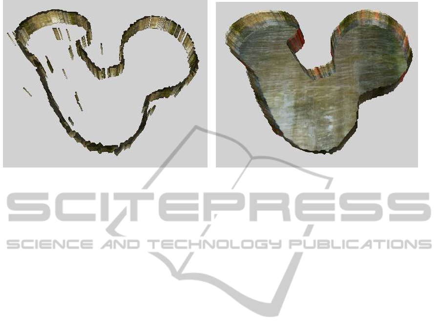
Figure 1: Geometric model extracted from an evidence grid created from sonar data. The model on the left is extracted
without application of our algorithm, while the model on the right has hole filling, pdf creation and uncertainty visualization
applied (red regions are less certain). This cistern is in a private home in Mdina, Malta.
pleted in the maritime setting (Pizarro et al., 2009)
and recent work in cenotes in Mexico (Fairfield et al.,
2010). Similar to the work to map cenotes (Fairfield
et al., 2010), this project involves the application of
marching cubes (Lorensen and Cline, 1987) to recon-
struct a geometric model of underwater data, however,
the cenote project relies on a very sophisticated and
significantly larger more expensive ROV and sensors
that would be impractical in water systems explored
in this project. Our research requires mapping in tun-
nels with passages and access points that are relatively
small (e.g. 0.30m diameter at some points), requiring
a micro ROV with low payload capacity and minimal
sensors (i.e. scanning sonar, depth sensor, and com-
pass).
Managing holes in acquired data is a mature
field with numerous research projects addressing hole
filling in both the surface and volumetric setting.
For an overview of many of the relevant research
projects related to polygonal repair, see the course
notes on ‘Geometric Modeling Based on Polyon-
gal Meshes’ (Botsch et al., 2007). Recent work
in surfaces has been conducted (Bac et al., 2008),
while seminal work in the volume setting includes,
VRIP (Curless and Levoy, 1996) and subsequently
volume diffusion (Davis et al., 2002), along with re-
cent work in the volume setting by (Janaszewski et al.,
2010). While there has been excellent work in the
field of hole filling, the work presented in this paper
addresses the unique challenge of acquired data from
noisy sonar along with the challenge of showing in-
formation regarding confidence in our filled geomet-
ric models.
Visualization and Uncertainty. For this project,
we use well established visualization techniques to
create visually appealing models and to convey uncer-
tainty (Pang et al., 1997; Schmidt et al., 2004). Uncer-
tainty visualization are relevant to many fields (Pang
et al., 1997; Schmidt et al., 2004; Pfaffelmoser et al.,
2011; Grigoryan, 2002). The work presented in this
paper contributes a method to statistically analyze and
quantify the certainty of filled regions that could then
be visualized with various uncertainty techniques.
Mapping via Underwater Robot Systems. This
project relies on data acquired from algorithms for
mapping with underwater robots, in particular, un-
der water Simultaneous Localization and Mapping
(SLAM) (e.g. (Williams et al., 2000), (Hern`andez
et al., 2009), and (Fairfield et al., 2006)). The work of
Thurn (Thrun et al., 2005) includes a good survey of
the core techniques capable of fusing data from mul-
tiple sensors to create maps.
3 ALGORITHMS AND PRACTICE
This work is focused on reconstructing geometric
models from evidence maps representing Mediter-
ranean water storage systems (cisterns, wells and wa-
ter galleries). Specifically, the space being mapped
is discretized into a two dimensional grid of cells
with given a likelihood p
i, j
∈ [0, 1] of being occupied
(Thrun et al., 2005) and (White et al., 2010). The ev-
idence grid is extrapolated into three dimensions to
the appropriate height of the water system, and can
then be treated as volume data, and geometric models
IVAPP2013-InternationalConferenceonInformationVisualizationTheoryandApplications
594
of the scanned data can be constructed via marching
cubes, similar to the work presented in (Forney et al.,
2011). Any cell with p
i, j
> t is considered an occu-
pied cell and associated with a wall in the model. The
threshold value, t, is used to define occupancy and is
generally set to values in the range .65 − .85. We re-
fer to cells in the grid at location (i, j) as x
ij
, and the
probability of that cell, p(x
ij
), as p
ij
.
Due to the acquisition process, gaps in the ev-
idence grid are common and can lead to unwanted
holes in the reconstructed models. See Figures 4
and 2, for examples of incomplete evidence grids that
lead to geometric models with many holes, like those
seen in Figures 1 and 6. As the acquired data is known
to represent water tight structures, hole filling is nec-
essary to construct more realistic models.
3.1 Hole Filling
In summary, for our setting, hole filling is achieved by
fitting a function, F, to the {x, y} position of a subset
of occupied cells surrounding identified holes. Next,
unfilled cells of the grid in the ‘hole’ that are crossed
by F are set to occupied in order to fill the hole. To vi-
sualize the effectiveness of our fitting method, we an-
alyze the accuracy of filled regions. For each model,
we execute a learning process on real data to compute
a pdf to represent the likelihood of the filled cell’s cer-
tainty as a function of neighboring cells being filled
and the distance from those cells.
3.1.1 Simulating Holes for Learning
Using acquired evidence grids, we wish to analyze
our hole filling on real data. We start by identify-
ing fairly complete sections of input data, represent-
ing walls of the water system. These walls are repre-
sented by long runs of connected occupied cells, into
which we introduce ‘simulated holes’. Specifically,
varying length valid segments of the evidence grid are
selected. A segment is a group of cells containing all
neighboring occupied cells. A neighboring cell is a
cell x
i±1j±1
. Valid segments have a minimum length,
l
min
, (in practice, l
min
= 9).
We create ‘simulated holes’ by knocking out the
middle section of valid segments by setting some
of the occupied cells in the segment to unoccupied.
When creating holes, we randomly choose segment
lengths to create a variety of hole sizes. This method
restricts our holes to a minimum size of around 3
cells, but allows them to be as large as a third of the
longest segment length. For the removed sections,
the occupied cells closest to the edge of the hole, one
from each side, are defined as endpoints, e
a
ij
and e
b
ij
.
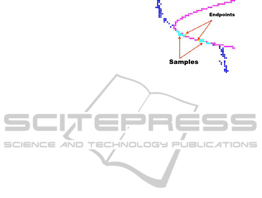
Figure 2: Definitions are shown in this figure from data
from the same cistern shown in Figure 1. Occupied cells
are shown in dark blue. Sample Points, S
S
are shown high-
lighted in light blue, endpoints are shown in orange and pink
samples, S
F
, correspond to a cubic polynomial fit to the hole
between the two endpoints. Only the sample points, S
H
that
lay between the two endpoints will be filled.
Endpoint detection and matching in practice is dis-
cussed in Section 3.2.
To fill each hole and measure the accuracy of each
fit, we define the following (see Figure 2):
1. The shortest distance between a cell, x
ij
and a
point on the fitted curve F, f
xy
as, kx
ij
− f
xy
k (for
higher order polynomials, this distance represents
the arc length along the curve).
2. S
S
is the set of occupied cells that were not re-
moved from the segment
3. F is the polynomial fit computed using Gauss-
Jordan elimination on set S
S
4. S
F
is the set of cells in the evidence grid that lay
on the fitted curve F
S
F
= {x
ij
| |x
i
− f
x
| < 0.5,
|x
j
− f
y
| < 0.5} (1)
5. S
H
is the subset of cells belonging to S
F
that lie
between the endpoints, e
a
i
and e
b
i
S
H
= {x
ij
| S
F
,
x
i
≤ max(e
a
i
, e
b
i
),
x
i
≥ min(e
a
i
, e
b
i
),
p
ij
< t} (2)
Given these definitions, in order to fill the ‘sim-
ulated hole’, the unoccupied cells from S
H
are set to
filled: ∀x
ij
∈ S
H
, p
ij
= 1.
All observed water storage systems contain rela-
tively smooth man-made walls, thus we found the use
of varying order polynomials (linear, quadratic, or cu-
bic) worked well (documented shortly), however, our
UncertaintyVisualizationandHoleFillingforGeometricModelsofAncientWaterSystems
595

algorithm does not depend on the structure or fitting
method of this function and any standard approach to
function approximation can be used.
3.1.2 Probability Distribution Function
Ideally, we would like to model the uncertainty of all
the filled cells in S
H
that we have introduced during
hole filling. To accomplish this, we can repeatedly
create simulated holes, then fill them and measure
their accuracy against the original data. This process
allows us to compute a probability distribution func-
tion, η(d
e
), that models the likelihood that any cell
x
ij
∈ S
F
has p
ij
> t, as a function of the distance d
e
from x
ij
to the nearest endpoint. That is, the pdf rep-
resents the likelihood that F sets the appropriate cells
to being occupied, depending on the distance from the
cell to the start of the hole.
η(d
e
) = P(p
′
ij
> t | d
e
, x
ij
∈ S
H
, p
ij
> t) (3)
To compute this pdf, we learn from the evidence
grids by tabulating a histogram of cells of the filled re-
gion that match the original data. We analyze each fit
by comparing the newly filled data with the ‘known’
real data. Specifically,for each cell x
ij
∈ S
H
, we check
to see if the cell from the original evidence grid also
had an occupied cell at the same x
ij
. This data is tabu-
lated into discrete bins, based on their distance along
F to the nearest endpoint to build up a histogram.
Specifically, for each unit along F, if the cell x
ij
cor-
responds with an occupied cell in the original data, we
consider this point a hit, if not it is a miss. Distances
along F, denoted as d
e
, are measured along the arc of
the fit from the nearest end point. For each type of fit:
linear, quadratic, and cubic, hits and misses are tallied
into discrete bins for each order polynomial.
We build up the histogram data by iteratively re-
peating hole filling of simulated holes for each dataset
per fit, and computing hits for each hole. Once the
samples have been collected, the percentage of hits
at given distances along the curves are computed for
each fit. See Figure 3 for an example of the discrete
binned distance values of a completed histogram for
one evidence grid for a quadratic fit. To create a con-
tinuous pdf for each model, the discrete binned hit
percentages at distances along the curve are fit with a
cubic polynomial.
The goal of this project is to reconstruct models
that will be used to illustrate the shape of water sys-
tems, and it is important to distinguish between the
portions of the model reconstructed from acquired
data and the geometry introduced during the hole fill-
ing, as well as the accuracy of the filled data. We use
each pdf in order to convey this information.
Figure 3: A histogram of tallied hits for a quadratic fit
for the Tas Silg evidence grid. Bins are discretized at arc
lengths zero to 5 along F (measured from either end point,
so the fewest hits are in the middle of the hole at a largest
distance of 5 units from either endpoint)).
3.1.3 Application of Pdf Data for Visualization
Once the pdf information has been computed for a
given model, the data can be applied to cells in the
hole filling process. When filling a hole, each filled
cell is assigned a probability based on it’s distance
from the closest endpoint, d
e
. The pdf for the specific
order polynomial chosen as the best fit is referenced
for certainty information and that data is assigned to
the newly filled cell. We describe the error metric
used for selecting the best fit in Section 3.2. Thus,
every newly filled cell is given a value, γ, which rep-
resents the predicted likely-evidence of that fit match-
ing the input model’s learned shape (or actual data).
We allow the user to visualize this uncertainty
by changing the coloring of the surface polygons for
those extracted from evidence cells with a value of γ.
For each vertex, red is added to the texture coloring
based on 1− γ, leading to less certain regions having
higher red colorings. Figures 1, 4, 7, and 6 all show
examples of the uncertainty visualizations generated
with our visualization system.
3.1.4 Validation
During this learning process, we also validate our hole
filling method overall. Specifically, we can tally over-
all the percentage of true positives, that is occupied
cells that we would fill using our method that were
originally occupied in the input data. We can also
compute false positives, cells that were unoccupied in
the original data but are filled via our hole filling. See
Table 1 for results of the statistical analysis for seven
models evaluating the results of hole filling. Note that
all models perform very well with an average of 83%
true positives and only 17% false positives. Over-
all for all data sets the computed true positives are
> 68%, with the most challenging data being a very
long water gallery with over 87 holes.
We have presented our method to statistically ana-
lyze our hole filling method and compute a pdf which
IVAPP2013-InternationalConferenceonInformationVisualizationTheoryandApplications
596
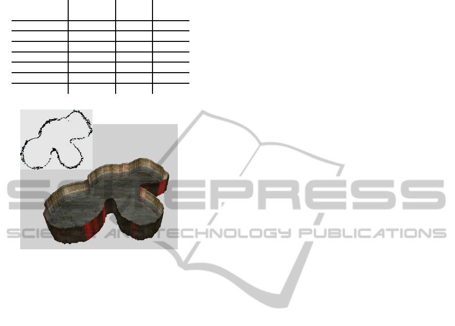
Table 1: Statistics for models.
Model name size positives false
of grid positives
Case Cutietta 120*120*26 94% 06%
College Garden 100*320*30 89% 11%
Gatto Pardo 132*109*25 75% 25%
Keyhole 150*100*30 87% 13%
Site 8 160*120*25 85% 15%
Tas Silg 187*175*26 83% 17%
Qanat 562*162*26 68 % 32%
Figure 4: The evidence grid and geometric model of the
Gatto Pardo cistern (private home in Mdina, Malta).
models the certainty of our hole filling, computed via
a learning process. We now describe how to apply our
hole filling to real holes in acquired data.
3.2 Hole Filling in Practice
For this expedition, investigators deployed a Video-
Ray ROV equipped with an underwater micron scan-
ning sonar, depth sensor, and two video cameras. The
ROV was lowered into cistern access points until it
was submerged. The investigators then tele-operated
the robot to navigate the underwater environment.
Due to the importance of acquiring accurate data, sta-
tionary sonar scans were takenusing a SeaSprite scan-
ning sonar mounted on top of the ROV. These sonar
measurements were used to generate evidence grids
that in turn, were used to generate geometric mod-
els of the cisterns (McVicker et al., 2012) and (White
et al., 2010), (Forney et al., 2011).
For real world acquired data, a number of subtle
challenges arise when applying hole filling to con-
struct a complete water tight model. In practice, we
find two types of holes that must be filled: those due
to under-sampling, characterized by very small neigh-
boring segments and those due to missing data, char-
acterized by larger holes between defined segments.
See Figures 2 and 7 for examples of both. We choose
to fill small holes first to build up information about
the shape of a model, thus we fill holes in an iterative
fashion with the smallest holes being filled first via a
distance threshold, E
τ
, that is expanded only after all
holes within that range are filled. Our algorithm for
filling holes involves the following steps:
for E
τ
= min;E
τ
< H;E
τ
+ +
Detect endpoints of valid segments
Match best pairs of endpoints
for any pairs with a size < E
τ
fill identified holes
Endpoint Detection. The first stage in hole filling
is identifying the segments in the evidence grid. The
evidence grid created from the sonar data may contain
segments of varying thickness due to the reflection of
the sonar’s wide cone shaped beam off of organically
shaped walls. When identifying the endpoints of seg-
ments, we cannot make assumptions about the seg-
ment’s cell’s connectivity or endpoint locations (See
Figure 2). In order to compute approximate segment
endpoints, we identify the start and end cells of long
sequences or paths of occupied cells using two passes
of Dijkstra’s algorithm. We have found two passes
of Dijkstra’s to suffice in practice to identify two rea-
sonable extremas of the segment to use as potential
endpoints. The algorithm proceeds as follows:
1. Using any occupied cell x
ij
as the starting point,
a Dijkstra’s search traverses the neighborhood of
grid cells, x
i±1, j±1
, connecting to any unvisited
occupied cell. The cell in the resulting graph
which is reached via the longest path is identified
as the first endpoint of the segment, e
1
ij
.
2. A second pass is run using this endpoint, e
1
ij
, as
the root node. The node at the end of the longest
path in this graph is identified as the second end-
point of the segment, e
2
ij
.
Endpoint detection proceeds until all occupied cells
in the evidence grid have been traversed. This method
may miss extrema for segments that branch, however,
it has been found to work well in practice.
To account for noise in the evidence grid, a seg-
ment is considered a valid segment only if the distance
from endpoint to endpoint along its Dijkstra’s graph is
≥ 4, and a valid endpoint is any endpoint belonging
to a valid segment. We refer to the length along a Di-
jkstra’s graph from cell a to cell b as D
d
(a, b) where
the cost of traversing to a neighboring occupied cell
(x
i±1, j±1
) is always 1. Once all valid endpoints have
been identified, we are ready to identify holes as the
cells with p
ij
< t that lie between pairs of valid end-
point. In order to fill these ‘holes’ (regions that are
unoccupied) properly, corresponding endpoints must
be identified and matched.
UncertaintyVisualizationandHoleFillingforGeometricModelsofAncientWaterSystems
597

Figure 5: Left: The complete geometric model of the Col-
lege Garden water system, including the correct reconstruc-
tion of three columns found in the cistern. Right: Evidence
grid and geometric model of Conca D’Oro Qanat.
Endpoint Matching. In practice, we do not know
which pairs of endpoints correspond to a hole and
matching endpoint pairs that are closest together is
not always accurate. Thus, given the collection of
endpoints, holes are identified via the use of pair-
wise testing, using two criteria: distance of end-
points to one another, and how well a given pair will
match the shape of neighboring segments. First, for
each iteration through the hole filling algorithm, end-
point matching is constrained to only potentially cre-
ate matches from any pair of endpoints, e
a
ij
and e
b
ij
whose Euclidean distance (ke
a
ij
− e
b
ij
k) < E
τ
.
Once the set of potential matches has been iden-
tified, the algorithm measures how well the fit of a
potential pair’s samples conforms to the local shape
of their segments. For each endpoint, all cells (from
the Dijkstra’s path) within a threshold distance, δ, are
identified as the endpoint’s sample points. The two
endpoint’s sample points are then fit with a polyno-
mial, F, (as in Section 3.1.1). The best matched fit
is the one with the smallest average distance from the
sample points to closest points on the fit, F.
In order to measure the best matched fit, S
S
is de-
fined in practice as the set of all cells of the evidence
grid that fall within a given distance, δ, of each end-
point, e
a
ij
and e
b
ij
. That is:
S
S
= {x
ij
| p
ij
> t,
D
d
(x
ij
, e
a
ij
) < δ ∨ D
d
(x
ij
, e
b
ij
) < δ} (4)
Given these definitions, the shape matching error
is computed as:
Min Err =
∑
∀x
ij
∈S
S
(kx
ij
− f
xy
k)
|S
S
|
(5)
Once all possible sets of endpoints have been
added to the list, we choose the matched endpoints
with the lowest error allowing each individual end-
point to be used only once. This matching process
allows us to identify the most likely endpoints that
correspond to a hole in the data.
Filling. Once best pairs of endpoints surrounding
holes have been identified, unoccupied cells within
holes are set to occupied by fitting the function F to
the sample data, S
S
, (defined above), for the best pair.
The order of F is chosen to minimize Min Err, (de-
fined above) and hole filling is applied as defined in
Section 3.1.1. That is, the unoccupied cells from S
H
are set to filled: ∀x
ij
∈ S
H
, p
ij
= 1.
Because F is determined by generating a func-
tion that matches local geometry, there must be well-
defined local geometry available in order to fill large
holes. Thus, we fill smaller holes first in order to build
up long segments in the evidence grid iteratively.
Final Visualizations. Once hole filling is complete,
the 2D evidence grid is extruded into 3D. The appro-
priate extrusion height is defined via measured data
from each specific water system site. The walls of the
water systems are well modeled by the evidence grid,
but in the surface creation stage a floor is added af-
ter hole filling by flood filling the interior of the now
closed model and adding an empty layer to the evi-
dence grid below the floor level. To remove small ex-
cess surface components due to noise (such as those
seen in Figure 1), volume smoothing is also applied
before surface extraction.
4 RESULTS
We have created geometric models for a dozen in-
dividual ancient water systems from the islands of
Malta, Gozo and Sicily. Each of these sites suffered
from incomplete data due to inaccuracies in the sonar
and mapping. These inaccuracies resulted in evidence
grids with numerous holes leading to extracted sur-
faces with holes. In this paper, we present a robust
hole filling algorithm, which fills in missing data in
the evidence grid, while honoring the shape of exist-
ing data. This hole filling algorithm results in water
tight meshes with boundary. We present the statistical
analysis used to validate this algorithm and to con-
struct a probability distribution function to model the
accuracy of the filled data. We also present details of
applying our hole filling method in practice. Using
the data gathered in our statistical analysis we also
present uncertainty visualizations of the filled surface
data. We believe this is the first such complete system
for mapping and reconstructing underwater geometric
IVAPP2013-InternationalConferenceonInformationVisualizationTheoryandApplications
598
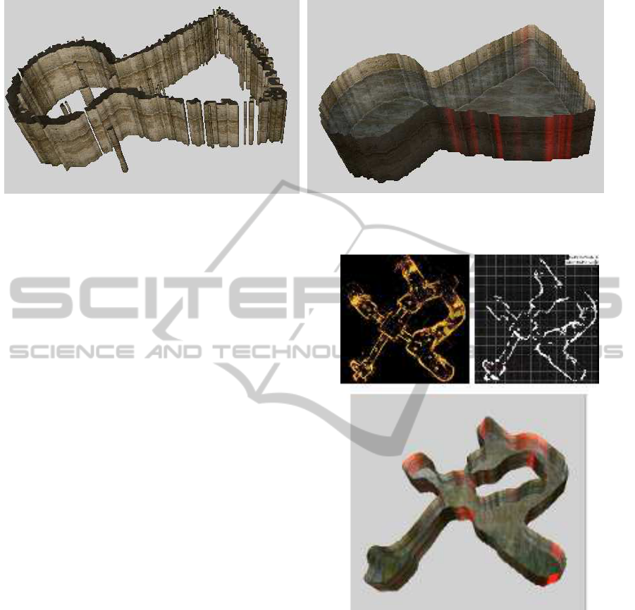
Figure 6: On the left is the geometric model of the House Dar T’ana (private home on Gozo) cistern before hole filling and
on the right is the complete geometric model including uncertainty visualization of surfaces created via hole filling.
structures with hole filling and uncertainty visualiza-
tions from evidence grids.
We show surface reconstruction results and un-
certainty visualization for six different ancient water
systems, (the physical scale of the grids in this paper
range from 0.03m to 0.1m per cell):
• Figure 1, shows the cistern located in a private
home on Gozo, (with 18 filled holes).
• Figure 4, shows the cistern located in a private
home in Mdina, Malta, (with 17 filled holes).
• Figure 7 shows results from sonar scans of the wa-
ter system at Tas Silg (Malta). This ancient water
system, located at the 2,000 year old temple site,
was over 15 meters long and very complex with a
loop structure connecting two entry points via two
divergent channels, (with 42 filled holes).
• Figure 5 is the cistern at Wignacourt Museum
College Garden (Malta). The cistern is fairly com-
plex and includes several chambers and three pil-
lars visible in the model, (with 20 filled holes).
• Figure 6 shows the cistern located at House Dar
Ta’Anna - Upper courtyard, Gozo, which is a key-
hole shaped cistern, (with 9 filled holes).
• Figure 5 shows the qanat at the hotel Conca d’Oro
(Sicily). This very long water gallery (over 40
meters long) was a part of the historic paper fac-
tory and data collection included over 20 station-
ary sonar scans (with 87 filled holes).
Table 1 includes information on the size of
datasets used for this work and information about the
accuracy of our hole filling data for each model. Note
that all datasets include numerous holes, up to 87 for
the qanat in the hotel Conca d’Oro.
Figure 7: The top row shows both the sonar data and the
evidence grid for Tas Silg. This very large water system
located on an ancient temple site was over 15 meters long.
The bottom image shows the complete geometric model,
including uncertainty visualization of filled holes.
4.1 Conclusions
We have presented a robust straight-forward hole fill-
ing algorithm, including statistical analysis of the cer-
tainty of filled regions and demonstrate resulting final
visualizations of the water systems. The hole filling
performs very well even with very noisy input data
and missing segments, while still preserving the orig-
inal shape of the input data (such as the small con-
necting tunnel in Tas Silg, (Figure 7).
UncertaintyVisualizationandHoleFillingforGeometricModelsofAncientWaterSystems
599

Future improvements to this work, include prop-
agating probability errors from the mapping process
into the evidence grid to visualize the certainty of the
acquired data itself, including, incorporating a model
of the sonar uncertainty more completely throughout
the reconstruction process as done in (Pandey et al.,
2007). Finally, some of the water systems explored
contain interesting shape variation in their vertical ex-
tent and 3D mapping is an active area of our work.
REFERENCES
Bac, A., Tran, N.-V., and Daniel, M. (2008). A multistep ap-
proach to restoration of locally undersampled meshes.
In GMP’08, pages 272–289.
Botsch, M., Pauly, M., Kobbelt, L., Alliez, P., L´evy, B.,
Bischoff, S., and R¨ossl, C. (2007). Geometric model-
ing based on polygonal meshes. In ACM SIGGRAPH
2007 courses. ACM.
Curless, B. and Levoy, M. (1996). A volumetric method
for building complex models from range images. In
SIGGRAPH ’96, ACM Press.
Davis, J., Marschner, S., Garr, M., and Levoy, M. (2002).
Filling holes in complex surfaces using volumetric
diffusion. In Symposium on 3D Data Processing, Vi-
sualization, and Transmission.
Fairfield, N., Kantor, G., Jonak, D., and Wettergreen, D.
(2010). Autonomous exploration and mapping of
flooded sinkholes. Int’l. J. Rob. Res., 29(6):748–774.
Fairfield, N., Kantor, G., and Wettergreen, D. (2006)). Real-
time SLAM with octree evidence grids for exploration
in underwater tunnels. In Journal of Field Robotics,
Vol 24, Issue 1-2, pp. 03-21.
Forney, C., Forrester, J., Bagley, B., McVicker, W., White,
J., Smith, T., Batryn, J., Gonzalez, A., Lehr, J., Gam-
bin, T., Clark, C., and Wood, Z. (2011). Surface recon-
struction of Maltese cisterns using ROV sonar data for
archeological study. In Proceedings of the 7th Int’t.
conference on Advances in visual computing.
Grigoryan, G. (2002). Probabilistic surfaces: Point based
primitives to show surface uncertainty. In Proceedings
Visualization 2002.
Hern`andez, E., Ridao, P., Ribas, D., and Batlle, J. (2009).
MSISPIC: A probabilistic scan matching algorithm
using a mechanical scanned imaging sonar. In Journal
of Physical Agents 3:311.
Janaszewski, M., Couprie, M., and Babout, L. (2010). Hole
filling in 3D volumetric objects. Pattern Recogn.,
43(10):3548–3559.
Lorensen, W. E. and Cline, H. E. (1987). Marching cubes:
A high resolution 3D surface construction algorithm.
In SIGGRAPH ’87, pages 163–169.
McVicker, W., Forrester, J., Gambin, T., Lehr, J., Wood, Z.,
and Clark, C. (2012). Mapping of ancient water stor-
age systems with an ROV for visualization: An ap-
proach based on fusing stationary scans within a par-
ticle filter. In IEEE ROBIO.
Pandey, A. K., Krishna, K. M., and Nath, M. (2007). Fea-
ture based occupancy grid maps for sonar based safe-
mapping. In Proceedings of the 20th Int’l. joint con-
ference on Artifical intelligence.
Pang, A. T., Wittenbrink, C. M., and Lodha, S. K. (1997).
Approaches to uncertainty visualization. The Visual
Computer, 13:370–390.
Pfaffelmoser, T., Reitinger, M., and Westermann, R. (2011).
Visualizing the positional and geometrical variability
of isosurfaces in uncertain scalar fields. In Computer
Graphics Forum (Proceedings of EuroVis 2011).
Pizarro, O., Eustice, R. M., and Singh, H. (2009). Large
area 3D reconstructions from underwater optical sur-
veys. IEEE Journal of Oceanic Engineering.
Schmidt, G. S., ling Chen, S., Bryden, A. N., Livingston,
M. A., Osborn, B. R., and Rosenblum, L. J. (2004).
Multidimensional visual representations for under-
water environmental uncertainty. IEEE Computer
Graphics and Applications, 24:2004.
Thrun, S., Burgard, W., and Fox, D. (2005)). Probabilistic
robotics. In MIT Press.
White, C., Hiranandani, D., Olstad, C., Buhagiar, K., Gab-
min, T., and Clark, C. (2010). The Malta cistern map-
ping project: Underwater robot mapping and localiza-
tion within ancient tunnel systems. In Journal of Field
Robotics.
Williams, S., Newman, P., Dissanayake, G., and Durrant-
Whyte, H. (2000)). Autonomous underwater simulta-
neous localization and map building. In Proceedings
of the 2000 IEEE Int’l. Conference.
APPENDIX
We wish to especially thank Christina Forney, Erik
Nelson, Jane Lehr and the ICEX teams (2011 &
2012). This material is based upon work supported by
the National Science Foundation, Grant No. 0966608.
IVAPP2013-InternationalConferenceonInformationVisualizationTheoryandApplications
600
