
On the Pitfalls of Desynchronization in Multi-hop Topologies
Clemens M¨uhlberger
Institute of Computer Science, University of W¨urzburg, Am Hubland, W¨urzburg, Germany
Keywords:
Desynchronization, Refractory Threshold, Self-organization, Wireless Sensor Network, Multi-hop Topology.
Abstract:
Biologically inspired self-organization methods can help to manage the access control to the shared commu-
nication medium of wireless ad-hoc networks. One lightweight method is the primitive of desynchronization,
which has already been implemented as MAC protocol for single-hop topologies successfully. Here, each
periodically transmitting node is able to establish a collision-free TDMA schedule autonomously. However,
multi-hop topologies are more realistic, but also more difficult to handle. For instance, the hidden terminal
problem is inherent in such topologies and complicates an implementation of this primitive as MAC proto-
col for multi-hop topologies: Each node requires knowledge about its two-hop neighborhood to establish a
collision-free TDMA schedule. Moreover, the problem of stale information is inherent in the primitive of
desynchronization and even could destabilize the whole system.
In this paper we describe our experience when extending a single-hop MAC protocol based on the primitive of
desynchronization for its usage within multi-hop topologies. During development, we identified some pitfalls
of desynchronization in multi-hop topologies, like stale information. As a result, we present our solution of a
self-organized MAC protocol based on the primitive of desynchronization for multi-hop topologies.
1 INTRODUCTION
Wireless ad hoc networks, and wireless sensor net-
works in particular, are characterized by their ability
to communicate wirelessly. All participating nodes
interact via a single shared medium. Access control
for this shared communication medium is a desirable
but also considerable task. The degree of difficulty of
such a task, amongst other things, depends on several
network parameters, like the network size (i.e., the
number of nodes), connectivity (i.e., the degree of the
nodes), or density (i.e., the ratio of number of extant
links to number of potential links). However, access
control is commonly intended to reduce the probabil-
ity of occurrenceof collisions. For this reason, several
protocols for medium access control (MAC) already
exist, mostly classified into contention-based carrier
sense multiple access (CSMA) and schedule-based
time division multiple access (TDMA). Within this
paper, we will focus on self-organized TDMA pro-
tocols, which divide the shared communication chan-
nel into several time slots providing exclusive access
for the actually assigned node. Such an assignment
requires coordination among the nodes. This coordi-
nation can be achieved, for instance, by explicit syn-
chronization of these time slots using a global clock,
which must then be provided by a dedicated base
node. Otherwise, the nodes must already have a priori
knowledge about the schedule of adequate time slots.
However, the centralized approach of synchronization
always involves a single point of failure, whereas a
fixed schedule (which is based on a priori knowledge)
is much too rigid and might be unable to handle topol-
ogy dynamics satisfactorily.
Instead, the biologically inspired primitive of
desynchronization as TDMA protocol for single-hop
topologies is proposed in (Degesys et al., 2007). One
main goal of such a self-organized MAC protocol us-
ing desynchronization is the avoidance of collisions,
even in the absence of both, a central scheduler as well
as the a priori coordination of the nodes. To achieve
this, each node calculates its next time of transmis-
sion autonomously. This computation is based solely
on locally available data, which makes the protocol
scalable, robust, and adaptive for single-hop topolo-
gies. Therefore, this MAC protocol is well suited for
ad hoc networks showing dynamics, variations, and
mobility.
The timeliness of the used data for an autonomous
decision making process is of utmost importance.
Since, however, self-adjustments by the nodes are
always made without any other node’s knowledge,
nodes could rely on potentially stale information.
This obsolete information might result in packet
99
Mühlberger C..
On the Pitfalls of Desynchronization in Multi-hop Topologies.
DOI: 10.5220/0004230900990108
In Proceedings of the 2nd International Conference on Sensor Networks (SENSORNETS-2013), pages 99-108
ISBN: 978-989-8565-45-7
Copyright
c
2013 SCITEPRESS (Science and Technology Publications, Lda.)

collisions or fluctuations of transmission time (cf.
Sect. 4.2). Finally, even the whole system could
destabilize. Indeed, this problem is inherent in the
primitive of desynchronization and is intensified at
multi-hop topologies due to a prolonged information
propagation. The expansion from single-hop to multi-
hop topologies further complicates the development
of a self-organized MAC protocol due to the so called
hidden terminal problem. This problem is inherent
in multi-hop topologies, and requires each node to
gain knowledge about its two-hop neighborhood for
a collision-free but self-organized communication.
The remainder of this paper is structured as fol-
lows: Section 2 formalizes the primitiveof desynchro-
nization as well as the emerging self-organized MAC
protocol for single-hop topologies, which builds the
basis for the MAC protocol analyzed herein. In
Section 3, we discuss problems and solutions aris-
ing when extending this MAC protocol from single-
hop to multi-hop topologies, e.g., the hidden terminal
problem. The pitfall of stale information, which is
inherent in the primitive of desynchronization, is an-
alyzed for single-hop as well as for multi-hop topolo-
gies in Section 4. Section 5 presents our lightweight
approach to cope with stale information in multi-hop
topologies: The impact of our new approach is dis-
cussed and a side effect is exemplified which helps to
solve emerging collisions in particular multi-hop sce-
narios. Next, we give a short survey of recent work
dealing with MAC protocols based on the primitive
of desynchronization in Section 6. Finally, Section 7
concludes the paper with a short outlook to future
work.
2 DESYNCHRONIZATION
This section describes the primitive of desynchroniza-
tion and introduces an implementation as MAC proto-
col for single-hop topologies. This formalization will
be the core for the following sections.
2.1 The Primitive of Desynchronization
Based on the first mathematical model of pulse-
coupled oscillators (Mirollo and Strogatz, 1990),
the biologically inspired primitive of desynchroniza-
tion (Degesys et al., 2007) implies that each node ”os-
cillates” at the same frequency f = 1/T. Applied to
the domain of wireless sensor networks, each node
tries to transmit a so called firing packet after every
period T. Such periodical data transmissions are com-
mon, for instance, in biomedical sensor networks due
to periodic sensor sampling (Støa and Balasingham,
2011).
Desynchronization is the ”logical oppo-
site” (Degesys et al., 2007) of synchronization,
i.e., each node tries not to perform its (periodic)
transmission at the same time, but instead at a
maximum temporal distance to all related nodes. For
single-hop topologies, in which each node reaches
each other node in a single hop, desynchronization
results in the temporally equidistant transmission
of firing packets: If such a network consists of a
set N of nodes, the time span between successively
transmitting nodes equals T/ |N|.
2.2 Desynchronization as MAC Protocol
The self-organized MAC protocol DESYNC (Degesys
et al., 2007) for single-hop topologies uses this
primitive of desynchronization. Each participat-
ing node can determine its next time of transmis-
sion within such a (fully connected) network au-
tonomously. Therefore, each node possesses a unique
identifier
1
i, and – as already mentioned before – each
node periodically transmits its firing packet.
To simplify the following analysis, we make some
(idealized) assumptions. First of all, the radio com-
munication range equals the interference range. Next,
all links are reliable and symmetrical. Moreover, each
node supports half-duplex mode, i.e., it can either
transmit or receive a packet at the same time. Finally,
each node has a finite buffer for (incoming) packets.
Let t
i
be the current time of firing of node i ∈ N,
and let t
+
i
be its next time of firing. When node
i finishes its period, it broadcasts its firing packet,
resets its phase, and updates t
+
i
. The phase shift
φ
i
(t) ∈ [0,T) of a node i denotes the elapsed time
since its current firing t
i
and the given point in time
t, normalized to the period T as
φ
i
(t) = (t − t
i
) mod T. (1)
Let N
1
(i) be the set of one-hop neighbors and let
d
i
= |N
1
(i)| be the degree of node i. Please note, for
(fully connected) single-hop topologies holds N
1
(i) =
N \ {i} and d
i
= |N| − 1 for every node i ∈ N. Every
time, node i receives a firing packet of its one-hop
neighbor j ∈ N
1
(i) at timet
j
, node i is able to calculate
the phase shift φ
i
(t
j
) towards this one-hop neighbor j
according to (1). For example, φ
i
(t
j
) = 0.5·T means
that node i has finished half of its current period when
node j transmitted its firing packet at time t
j
.
1
For the sake of simplicity, we do not further distinguish
between the identifier itself and the node’s ordinal in N.
Moreover, without loss of generality let 1 ≤ i ≤ |N|.
SENSORNETS2013-2ndInternationalConferenceonSensorNetworks
100

t
i
t
+
s(i)
t
p(i)
t
+
p(i)
t
+
i
s(i)
fir ing
i
p(i)
T
ϕ t
p(i) i
( )
(a) At time t
i
, node i is fir-
ing. It calculates the phase shift
φ
p(i)
(t
i
) and schedules its next
firing at t
+
i
, according to (3).
fir ing
α·ε
i
ϕ
i
(t
s(i)
)
t
i
t
s(i)
t
+
p(i)
t
p(i)
t
+
i
i
s(i)
p(i)
(b) At time t
s(i)
, successor s(i)
of node i is firing. Node i calcu-
lates the phase shift φ
i
t
s(i)
.
t
i
t
s(i)
t
+
i
i
firing
p(i)
s(i)
t
p(i)
α·ε
i
(c) At time t
p(i)
, predecessor
p(i) of node i is firing. Node i
has to record this time t
p(i)
.
t
i
t
+
i
fi r ing
ϕ
i
(t
s(i)
)
t
s(i)
i
p(i)
s(i)
t
p(i)
ϕ
p(i)
(t
i
)
(d) Now, t
+
i
is reached and be-
comes t
i
. The next steps corre-
spond to Figure 1(a).
Figure 1: Snapshots of the desynchronization process from node i’s point of view. Nodes move clockwise on the circle at
frequency f = 1/T with period T.
Two neighbors of node i are of special interest for
the DESYNC algorithm: The successive phase neigh-
bor s(i) ∈ N (successor) and the previous phase neigh-
bor p(i) ∈ N (predecessor). The successor broadcasts
its firing packet just after, whereas the predecessor
broadcasts its firing packet just before node i (cf. Fig-
ure 1(b) and Figure 1(c), respectively).
The primitive of desynchronization forces each
node to transmit its firing packet at a maximum tem-
poral distance towards both phase neighbors, i.e.,
each node attempts to achieve the midpoint of its
phase neighbors. Therefore, each node just has to
observe the firing packets of its phase neighbors s(i)
and p(i) to calculate the corresponding phase shifts
φ
i
t
s(i)
and φ
p(i)
(t
i
). Using both phase shifts, node i
is able to compute its adjustment factor ε
i
as
ε
i
=
φ
i
t
s(i)
− φ
p(i)
(t
i
)
2
. (2)
Finally, each node is able to set its next (absolute)
time of firing t
+
i
as
t
+
i
= t
i
+ T + α· ε
i
= t
i
+ (1− α) ·T + α· (ε
i
+ T).
(3)
The jump size parameter α ∈ [0, 1] regulates how fast
node i moves toward the assumed midpoint between
its phase neighbors p(i) and s(i). The endpoints of
this interval will not be considered within this paper,
since α = 0 means no movement at all, whereas α = 1
forces the nodes always to jump onto the current mid-
point of its phase neighbors without any damping.
One achieves good results using α = 0.95 as damping
factor (Degesys et al., 2007). The last expression of
(3) shows its similarity to the exponentially weighted
moving average, which smooths out short-term fluc-
tuations but highlights long-term trends.
If each node i respects the same (temporal) dis-
tance to its phase neighbors (i.e., ε
i
= 0), the stable
state of desynchrony is reached. Once, the system is in
stable state, the transmission times do not change any-
more – apart from clock drifts and topology changes.
3 DESYNCHRONIZATION IN
MULTI-HOP TOPOLOGIES
In Section 2, we presented the basic idea of a MAC
protocol for periodically transmitting nodes within a
single-hop topology. However, using this MAC pro-
tocol for multi-hop topologies is rather difficult. To
be consistent with the primitive of desynchroniza-
tion and to permit a collision-free communication
in multi-hop topologies, each node i additionally re-
quires knowledge about its set of two-hop neighbors
N
2
(i) (Degesys and Nagpal, 2008). Please note that
{i}, N
1
(i), and N
2
(i) are pairwise disjoint for every
node i ∈ N. Therefore, this section outlines the main
problems and solutions, when extending the MAC
protocol based on the primitive of desynchronization
from single-hop to multi-hop topologies.
3.1 Hidden Terminal Problem
The so called hidden terminal problem (Tobagi and
Kleinrock, 1975) is inherent in multi-hop topologies.
Suppose, a network consisting of three nodes a, b, and
c. Nodes a and c can directly communicate with node
b, but both nodes a and c are unaware of each other.
If at about the same time node a as well as node c
transmit a packet to node b, both radio packets collide
and node b receives just corrupt data – if any. Both
nodes a and c are hidden from each other, hence they
cannot overcome this packet collision using carrier
sense (CS) right before their transmissions.
OnthePitfallsofDesynchronizationinMulti-hopTopologies
101

One technique to solve the hidden terminal prob-
lem for contention-based CSMA protocols (Karn,
1990; IEEE, 2007) is the RTS/CTS handshake: If
node a wants to transmit data to node b, node a ini-
tially sends a request–to–send (RTS) to node b. If
node b received the RTS from node a correctly, node b
in return has to respond with a clear–to–send (CTS).
If node a correctly received this CTS, the RTS/CTS
handshake was successful and node a may start to
transmit data towards node b. However, our primitive
of desynchronization follows a self-organizing man-
ner which results in a schedule-based TDMA proto-
col. Therefore, the RTS/CTS handshake protocol is
quite incompatible with it.
3.2 The Local Max Degree
As already mentioned, each node requires addi-
tional knowledge about its two-hop neighborhood
to solve the hidden terminal problem in multi-hop
topologies. A compact and efficiently obtainable
information might be the local max degree D
i
=
max
d
j
| j ∈ N
1
(i) ∪ {i}
of a node i. Further, let
D
N
= max{D
i
| i ∈ N} be the global max degree.
With it, there exists a desynchronization algorithm,
which divides the period T into 2· (D
i
+ 1) slots and
converges in O (D
N
log|N|) periods with high proba-
bility (Motskin et al., 2009). However, approximately
half of the provided slots will remain unassigned. Fur-
thermore, the propagation (i.e., flooding) of the global
max degree D
N
causes high communication costs.
In single-hop and acyclic multi-hop topologies,
the provably minimal number of required time slots
per period for a collision-free communication within
the interference range of node i is D
i
+ 1. The M-
DESYNC algorithm (Kang and Wong, 2009) is also
based on the local max degree D
i
. However, the
M-DESYNC algorithm tries to maximize the slot uti-
lization, i.e., to get along with the minimal num-
ber of required slots D
i
+ 1. Therefore, each node
i has to exchange information about its degree d
i
with all its one-hop neighbors first. After this maybe
lengthy
2
exchange stage, each node i obtained knowl-
edge about its local max degree D
i
. Next, while
there are still conflicts, each node i selects one of
the D
i
+ 1 prioritized time slots. However, the M-
DESYNC algorithm is not very flexible, since each
topology change demands for both the lengthy ex-
change stage as well as for the competitive selection
stage. Furthermore, the M-DESYNC algorithm is not
applicable for cyclic multi-hop topologies (Kang and
Wong, 2009; M¨uhlberger, 2010).
2
There is just a contention-based back-off algorithm for
this exchange phase suggested (Kang and Wong, 2009).
3.3 The Phase Shift Propagation
The propagation of (relative) phase shifts is an-
other simple solution to obtain knowledge about
the two-hop neighborhood (Degesys and Nagpal,
2008). Regarding the primitive of desynchronization,
this approach was first implemented as EXTENDED-
DESYNC algorithm (M¨uhlberger and Kolla, 2009):
If each node propagates within its firing packet the
complete set of its one-hop neighbors together with
their (relative) phase shifts, each receiving node in
turn is able to assemble its two-hop neighborhood au-
tonomously. That means, each node i broadcasts (the
identifiers of) all its (currently known) one-hop neigh-
bors j ∈ N
1
(i) together with their relative
3
phase shifts
φ
i
(t
j
).
In comparison to the M-DESYNC algorithm, no
preliminary exchange phase is required. Instead, each
newly joining node just has to listen for a couple
of periods to make itself familiar with its neighbor-
hood before transmitting its first firing packet. There-
fore, the EXTENDED-DESYNC algorithm is robust
and reacts quickly on topology changes. However,
each node broadcasts its whole one-hop neighbor-
hood, which takes bandwidth and energy for algo-
rithmic purposes. Furthermore, the packet overhead
increases linearly with the size of the one-hop neigh-
borhood, i.e., a node with high degree has to trans-
mit more data in its firing packets and thus consumes
more bandwidth and more energy than a node with
low degree. This dependencywill also specify a lower
bound for the applied period T (M¨uhlberger, 2009).
3.4 Further Observations
Since the phase shift propagation is universally ap-
plicable and more flexible than the local max degree
approach, we will use the EXTENDED-DESYNC al-
gorithm as basis for our further analysis on multi-
hop topologies. However, regarding the primitive of
desynchronization for multi-hop topologies the fol-
lowing difficulties can be observed:
• All nodes share the same communication
medium, but a node i may just have local and
limited knowledge about the multi-hop network
(cf. Section 3.1).
• Therefore, the nodes in multi-hop topologies need
not to have equal degree anymore, but the degree
of a node i is at most d
i
≤ |N|− 1 (cf. Section 2.2).
• Hence, the time span between successively trans-
mitting nodes in multi-hop topologies might not
equal T/|N| anymore (cf. Section 2.1).
3
From the point of view of the current sender i.
SENSORNETS2013-2ndInternationalConferenceonSensorNetworks
102

• Furthermore, for multi-hop topologies, the phase
neighbors of node i might be two-hop neighbors
as well, i.e., p(i),s(i) ∈ N
1
(i) ∪ N
2
(i).
• Finally, between two nodes i, j ∈ N in single-hop
topologies holds the correlation i = p( j) ⇔ j =
s(i). For multi-hop topologies, this successor–
predecessor correlation needs not to hold any-
more.
4 PITFALL: STALE
INFORMATION
The primitive of desynchronization aims for a self-
organized but collision-free arrangement of time
slots. Hence, the nodes are able to rely on just lo-
cally available information, which can be both self-
provided and self-acquired. Consequently, received
data from adjacent nodes sometimes is ”stale”, i.e.,
the information obtained from received firing packets
might be obsolete at the time of its application, and
thus unreliable or even invalid. This problem already
exists in single-hop topologies. But it is intensified in
multi-hop topologies and will be described in detail
throughout this section.
4.1 Single-hop Topologies
Using the primitive of desynchronization, the prob-
lem of stale information is inherent in single-hop (as
well as multi-hop) topologies (Degesys et al., 2007):
While node i calculates its next time of firing t
+
i
ac-
cording to (3), its two phase neighbors might already
have adjusted their individual next time of firing au-
tonomously. Therefore, the formerly measured phase
shifts φ
i
t
s(i)
and φ
p(i)
(t
i
) might already be stale, es-
pecially if node i adjusts its next time of firing imme-
diately after transmitting its own firing packet at time
t
i
(cf. Figure 1). That means, node i estimates its next
time of firing t
+
i
on the basis of potentially unreliable
information, here the time of firing of its phase neigh-
bors.
In fact, the use of more recent data for the phase
shift φ
i
t
s(i)
in (3) will omit at least one unreliable in-
formation (Patel et al., 2007). For this purpose, node
i just has to calculate its next time of firing t
+
i
not im-
mediately after the transmission of its firing packet,
but immediately after the reception of the first subse-
quent firing packet of its successor s(i). As a result,
node i uses more recent data, but the equation (3) to
compute the next time of firing t
+
i
remains the same.
Just the time when the next time of firing is calculated
was delayed from t
i
to t
s(i)
.
4.2 Multi-Hop Topologies
For multi-hop topologies, this problem of obsolete fir-
ing information is intensified due to the hidden termi-
nal problem (cf. Section 3.1). Therefore, each node i
additionally must take care of its two-hop neighbors.
That means, each node i has to arrange itself accord-
ing to the firings of both its one-hop and two-hop
neighbors N
1
(i) ∪ N
2
(i) (cf. Section 3.4). However,
node i gains information about a two-hop neighbor
k ∈ N
2
(i) ∩ N
1
( j) just in cooperation with the corre-
sponding one-hop neighbor j ∈ N
1
(i). This data flow
from node j to node i is additionally delayed by at
least the phase shift φ
k
(t
j
) between the nodes j and k.
To exemplify the impact of stale information in
multi-hop topologies, we simulated a small but man-
ageable scenario by using a self-developed simulator
on an Intel Core i5 CPU with 2.60 GHz and 8.00 GB
main memory under the Windows 7 Professional 64
Bit operating system.
First, we assume idealized conditions, i.e., all
communication links are symmetrical and reliable,
not any node will fail, and there is no clock
drift. Next, the jump size parameter is set to α =
0.95 (Degesys et al., 2007). The simulated ”dumb-
bell” topology M
7
is easy to understand: It consists
of the set N = {1, . ..,7} of nodes as shown in Fig-
ure 2. This topology contains two cyclic (and com-
plete) sub-graphs C
3
= {1,2, 3} and C
′
3
= {4,5, 6}.
Let the nodes of both disjoint single-hop topologies
C
3
and C
′
3
start first. Therefore, both sub-graphs will
desynchronize independently, since they are unaware
of each other. Just when node 7 joins the network,
it successively gathers knowledge of both topologies
4
C
3
andC
′
3
. Node 7 connectsC
3
andC
′
3
with its first fir-
ing packet containing its one-hop neighborhood (i.e.,
nodes 1 and 4), and thus completes the topology M
7
.
Figure 3(a) shows the first 100 periods after the start
up of node 7 at period 45 from its point of view. Due
to the stale information in this multi-hop topology,
the one-hop and two-hop neighbors of node 7 (i.e, all
nodes of C
3
and C
′
3
) rather diverge than converge, as
intended by the primitive of desynchronization. In
fact, approximately 20 periods after the start up of
node 7, the time of transmission of each node fluctu-
ates with a constant but individual amplitude. More-
over, the phase neighbors of node 7 are its two-hop
neighbors node 6 and node 2 (cf. Section 3.4).
4
See Section 5.4 for the extremely rare case that the time
of firing of node 1 and node 4 are synchronized, i.e., t
1
= t
4
.
OnthePitfallsofDesynchronizationinMulti-hopTopologies
103

3
2
1 4
7
6
5
Figure 2: The ”dumbbell” topology M
7
consists of the set
N = {1, . ..,7} of nodes.
5 MULTI-HOP SOLUTION FOR
DEALING WITH STALE
INFORMATION
In Section 4, we analyzed the problem of stale infor-
mation. As already mentioned, this problem is inher-
ent in the primitive of desynchronization. For single-
hop topologies it is sufficient for a node i to calcu-
late its next time of transmission t
+
i
after receiving
the firing packet of its successor s(i) (cf. Section 4.1).
Therefore, we will focus on multi-hop topologies in
this section. However, we cannot avoid stale infor-
mation at all, but with our new approach we want to
take control of its evolution and reduce its impact in
multi-hop topologies.
5.1 Refractory Threshold
In multi-hop topologies, the effect of stale informa-
tion is intensified due to the delayed propagation
of information about two-hop neighbors (cf. Sec-
tion 4.2). To some extent, our approach follows the
law of similars, because we suggest to intentionally
delay the adjustment of a node’s next time of fir-
ing. Therefore, we introduce an additional refractory
threshold ρ ∈ [0,1] along with a continuous random
variable X
i
∈ [0,1] following the continuous uniform
distribution U (0,1). According to the random vari-
able X
i
, the adjustment factor ε
i
will be considered,
and node i will set its next time of firing t
+
i
as
t
+
i
=
t
i
+ T + α·ε
i
ρ < X
i
(4a)
t
i
+ T otherwise (4b)
Obviously, choosing ρ = 0 lets the nodes always ad-
just their time of firing, which results in the same be-
havior as described in Section 4.2. In contrast, choos-
ing ρ = 1 is useless, since a node will not use its ad-
justment factor according to (2) for its next time of
firing anymore.
In some sense, the refractory threshold ρ contra-
dicts the primitive of desynchronization, because it
”skips” the adjustment of the next time of firing us-
ing (2). However, it allows a node to keep its phase
(and thus its time of firing) with a probability of ρ.
Nevertheless, this behavior helps the system to con-
verge: Let node i be phase neighbor of another node
j ∈ N
1
(i) ∪ N
2
(i). According to Section 3.4, node j
in turn needs not to be phase neighbor of node i. If
node i skips the adjustment of its phase using (4b),
node j’s estimation of its next time of firing remains
valid regarding the phase shift towards node i. The
information about node i remains reliable.
5.2 Algorithmic View
To explain the algorithmic view of our refractory
threshold, we present pseudo-code of our approach
to omit stale information in multi-hop topologies in
Listing 1. Of course, this pseudo-code is based on the
phase shift propagation (cf. Section 3.3).
1 // upon firing:
2 if
(firingTimerExpired ()) {
3
setFirstPacketReceived (true);
4
transmitFiringPacket ();
5 t
i
=
now();
6 t
+
i
= t
i
+ T
;
7 φ
p(i)
(t
i
) = (t
i
− t
p(i)
)
%
T
;
8
setFiringTimer (
t
+
i
);
9
}
10 // upon receiving firing packet:
11 if
(isFirstPacketReceived ()) {
12
setFirstPacketReceived (false);
13 t
s(i)
=
now();
14 t
p(i)
=
now();
15 φ
i
t
s(i)
= (t
s(i)
− t
i
)
%
T
;
16 ε
i
= 0
;
17 if
(
ρ <
Random.nextDouble()) {
18 ε
i
=
φ
i
t
s(i)
− φ
p(i)
(t
i
)
/2
;
19
}
20 t
+
i
= t
i
+ T + α·ε
i
;
21
setFiringTimer (
t
+
i
);
22
}
else
{
23 t
p(i)
=
now(); }
24
}
Listing 1: Pseudo-code with integrated refractory threshold
ρ.
If the firing timer of node i is expired (cf. Listing 1,
line 2), node i transmits its firing packet (cf. l. 4) at
time t
i
(cf. l. 5). Due to the fact that the link between
transmitter and receiver could be unreliable (e.g., the
former transmitter might have left the network or ran
out of energy, or a collision occurred at the receiver
due to a newly joining node) node i cannot predict
if there (once again) will be a successor transmitting
a firing packet. Therefore, by reasons of precaution,
node i has to schedule (cf. l. 8) its next time of firing as
SENSORNETS2013-2ndInternationalConferenceonSensorNetworks
104

t
+
i
= t
i
+ T (cf. l. 6). Node i uses this scheduled time
of firing if it does not receive any other firing packets.
Otherwise, node i is receiving another firing packet
(cf. ll. 10–24) before its firing timer expires again.
If node i receives the first subsequent firing packet
(cf. l. 11) of its successor s(i) at t
s(i)
(cf. l. 13), it cal-
culates the current phase shift towards its successor
(cf. l. 15). Since successor and predecessor of node
i could be the very same neighbor node, node i also
sets t
p(i)
here (cf. l. 14). If the refractory threshold is
less than a continuous random value (cf. l. 17), node i
calculates its adjustment factor ε
i
(cf. l. 18). Anyway,
node i updates the (already scheduled) next time of
firing t
+
i
(cf. l. 20) and sets its firing timer (cf. l. 21).
Otherwise, if the currently received firing packet is
not the first subsequent firing packet, it could origi-
nate from node i’s predecessor p(i). Therefore, node
i has to set t
p(i)
precautionary (cf. l. 23).
5.3 Simulation Results
We will exemplify the impact of our new threshold
on the simple scenario from Section 4.2, where the
two disjoint single-hop topologiesC
3
andC
′
3
are com-
bined by node 7 (cf. Figure 2). Again, we use the self-
developed simulator on the same computer as well as
the idealized conditions as mentioned in Section 4.2.
As suggested in literature (Degesys et al., 2007), we
set α = 0.95 again.
However, this time, each node calculates its next
time of firing according to (4) using ρ = 0.25. That
means, on average each node keeps its phase at every
fourth period. In contrast to the scenario described
in Section 4.2, which results in fluctuating time of
transmission of each node (cf. Figure 3(a)), the re-
fractory threshold now helps the network to converge
after about 25 periods since the start up of node 7 (cf.
Figure 3(b)). Moreover, the phase neighbors of node
7 again are its two-hop neighbors node 6 and node 2
(cf. Section 4.2).
Notably, a larger refractory threshold slows down
the convergence rate: In comparison to the scenario
described above, we just raised the refractory thresh-
old to ρ = 0.9. The simulation result is shown in Fig-
ure 3(c): The refractory threshold is clearly set too
high, but still the network is approximately desyn-
chronized after about 50 periods since the start up of
node 7. In comparison to the previous simulation re-
sults, the phase neighbors of node 7 have changed to
its two-hop neighbors node 2 and 5.
On the other hand, if the refractory threshold is set
too low, the system rather diverges than converges.
For instance, if we set ρ = 0.1 at the same scenario
from above, the time of transmission of each node
1
0
25
50
75
100
40 50 60 70 80 90 100 110 120 130 140 150
rel. phase [in %]
time [in #periods]
6
3
4
5
2
(a) Without our refractory threshold, i.e., ρ = 0.
3
2
1
4
6
5
0
25
50
75
100
40 50 60 70 80 90 100 110 120 130 140 150
rel. phase [in %]
time [in #periods]
(b) With our refractory threshold ρ = 0.25.
3
2
1
4
6
5
0
25
50
75
100
40 50 60 70 80 90 100 110 120 130 140 150
rel. phase [in %]
time [in #periods]
(c) With our refractory threshold ρ = 0.9.
3
2
1
4
6
5
0
25
50
75
100
40 50 60 70 80 90 100 110 120 130 140 150
rel. phase [in %]
time [in #periods]
(d) With our refractory threshold ρ = 0.1.
Figure 3: Simulation of M
7
(about 110 periods since the
start up of node 7 at period 45), α = 0.95, point of view:
node 7.
again fluctuates, but with a smaller amplitude (cf. Fig-
ure 3(d)).
The simulation results so far exemplify the capa-
OnthePitfallsofDesynchronizationinMulti-hopTopologies
105
bility of our refractory threshold. Indeed, to have a
substantial impact, the refractory threshold must ex-
ceed a certain value according to the particular topol-
ogy and start up scenario. However, the refractory
threshold ρ must be set carefully in combination with
the jump size parameter α (cf. Section 7).
5.4 Side Effect
Our refractory threshold obviously introduces a prob-
abilistic component. This component can also help
to solve emerging collisions in multi-hop topologies.
Therefore, to exemplify the impact of our refractory
threshold on emerging collisions, we slightly mod-
ify the simple scenario from Section 4.2, where the
two disjoint single-hop topologiesC
3
andC
′
3
are com-
bined by node 7 (cf. Figure 2). Again, we use the self-
developed simulator on the same computer as well as
the idealized conditions as mentioned in Section 4.2.
This time, we synchronize the start up sequence of the
subgraphsC
3
and C
′
3
, i.e., nodes 1 and 4 start up at the
same time, nodes 2 and 5 start up at the same time,
and node 3 and 6 start up at the same time.
First, we set α = 0.95 and ρ = 0, i.e., we make no
use of our refractory threshold (cf. Section 5.1). As
expected, the disjoint single-hop topologies C
3
and
C
′
3
will desynchronize independently. However, due
to the idealized conditions and the lack of any prob-
abilistic component, nodes 1 and 4 have chosen the
very same time of firing. That means, when node 7
starts up and tries to join the network, all firing pack-
ets of node 1 and 4 collide at node 7 due to the hid-
den terminal problem. Therefore, node 7 receives just
corrupt data, and thus is not able to gain any knowl-
edge about the topologiesC
3
and C
′
3
. In contrast, both
nodes 1 and 4 receive the empty firing packets of node
7, but thus remain unaware of each other (cf. Sec-
tion 3.1).
The start up sequence of the subgraphs C
3
and C
′
3
remains synchronized as described above. But now,
we increase the refractory threshold ρ = 0.25, and
thus activate our probabilistic component. Therefore,
the disjoint single-hop topologies C
3
and C
′
3
will still
desynchronize independently. However, even though
both nodes 1 and 4 had the same start up time, their
time of firing drift apart with high probability. That
means, when node7 joins the network, it nowreceives
the firing packets of both nodes 1 and 4. With its first
firing packet containing both one-hop neighbors (i.e.,
nodes 1 and 4), node 7 connects C
3
and C
′
3
, and thus
completes the ”dumbbell” topology M
7
again. Fig-
ure 4 shows about the first 110 periods from the point
of view of node 1 since its start up at period 1.
3
2
4
7
0
25
50
75
100
0 10 20 30 40 50 60 70 80 90 100 110
rel. phase [in %]
time [in #periods]
Figure 4: Simulation of M
7
(about 110 periods since the
start up of node 1 at period 1), α = 0.95, ρ = 0.25, point of
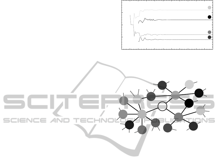
view: node 1.
82
87
24
57
15
23
78
58
86
51
9
99
33
83
19
62
27
40
Figure 5: One-hop and two-hop neighborhood of node 82
of topology R
100
, consisting of the set N = {1,...,100} of
nodes.
5.5 Scalability Test
To demonstrate the scalability of our new approach,
we simulated a more complex scenario by our self-
developed simulator under the idealized assumptions
from Section 4.2. This time, the topology R
100
con-
sists of the set N = {1,.. .,100} of nodes. Symmetri-
cal links between nodes are set randomly. Each node
starts up randomly within the first period. Since our
analysis will focus on node 82, Figure 5 just shows
the one-hop and two-hop neighbors of node 82 within
the observed topology R
100
.
First, we set α = 0.95 and ρ = 0, i.e., we make
no use of our refractory threshold (cf. Section 5.1).
As already observed in Section 4.2, the time of trans-
mission of each node fluctuates, i.e., the one-hop and
two-hop neighborsof node 82 rather divergethan con-
verge (cf. Figure 6(a)).
If we just increase the refractory threshold ρ =
0.25, the system converges after about period 75 (cf.
Figure 6(b)). If each node keeps its phase at ev-
ery fourth period on average, the network is well
desynchronized, although the network consists of 100
nodes. Therefore, our approach not only scales well
with the network size, but it is also suitable for large
networks.
SENSORNETS2013-2ndInternationalConferenceonSensorNetworks
106

0
25
50
75
100
0 10 20 30 40 50 60 70 80 90 100 110
rel. phase [in %]
time [in #periods]
(a) Without our refractory threshold,i.e., ρ = 0.
0
25
50
75
100
0 10 20 30 40 50 60 70 80 90 100 110
rel. phase [in %]
time [in #periods]
(b) With our refractory threshold ρ = 0.25.
Figure 6: Simulation of R
100
(about 110 periods since the
start up of node 82 at period 1), α = 0.95, point of view:
node 82.
6 RELATED WORK
In the previous sections, we have already referred to
work regarding the primitive of desynchronization.
Therefore, this section describes further work dealing
with the primitive of desynchronization as MAC pro-
tocol, or with the refractory treatment of information.
6.1 Refractory Period
In Section 5, we have introduced our refractory
threshold ρ to handle obsolete and potentially unre-
liable data from neighbor nodes. Therefore, a node
probabilistically skips the adjustment of its next time
of transmission to provide more reliable data. Sim-
ilar to our approach is the so called refractory pe-
riod (Degesys et al., 2008), which helps to synchro-
nize (not to desynchronize, as we do) strongly pulse-
coupled oscillators: If an oscillator receives the firing
of a neighbor within the refractory period, the receiv-
ing oscillator does not process this incoming firing.
That means, the phase shift between sender and re-
ceiver is too short to be considered, and thus, the re-
ceiver temporarily does not adjust its next time of fir-
ing. Moreover,the phase shift between two oscillators
specifies in this approach, whether an oscillator skips
the adjustment of its next time of firing or not. In
contrast, our refractory threshold is probabilistic and
independent from the phase shift between two nodes.
6.2 Artificial Force Field
Another approach to desynchronize a single-hop net-
work is the DWARF algorithm (Choochaisri et al.,
2012), which mainly reduces the impact of erroneous
information from phase neighbors. Thus, the next
time of firing of a node i does not only depend on the
firings of its phase neighbors. Instead, the next time
of firing is specified by an artificial force field which
is defined by all other nodes. Each force is weighted
by the phase shift of the corresponding neighbor node
towards the adjusting node i. This approach is very ef-
ficient for single-hop topologies. It also results in the
equal time span T/|N| between successively trans-
mitting nodes. However, to the best of our knowl-
edge, an extension for multi-hop topologies is cur-
rently missing.
6.3 Orthodontics-inspired Approach
The orthodontics-inspired algorithm (Taechalertpais-
arn et al., 2011) makes use of the fact that the time
span between successively transmitting nodes within
a single-hop topology equals T/ |N|. Therefore,
knowing |N|, each node can decide autonomously,
if it is already desynchronized, i.e., adequately ar-
ranged, or if it still has to adjust its next time of firing.
Each already desynchronized node simply keeps its
phase. With it, the impact of obsolete information is
reduced. However, due to the observations in Sec-
tion 3.4, this approach is not applicable for multi-hop
topologies.
7 CONCLUSIONS AND
OUTLOOK
In this paper we described the biologically inspired
primitive of desynchronization as MAC protocol
for wireless sensor networks. The resulting self-
organized protocol for single-hop as well as for multi-
hop topologies has to manage the problem of stale
information as well as the hidden terminal problem.
Due to these problems, the periodical transmission
times of the nodes may fluctuate in a multi-hop topol-
ogy. Therefore, we installed the refractory thresh-
old ρ. According to this threshold, and contrary to
the primitive of desynchronization, each node is now
able to probabilistically skip the adjustment of its next
OnthePitfallsofDesynchronizationinMulti-hopTopologies
107

time of firing. Based on some sample scenarios, we
demonstrated the impact of our approach for a small
but manageable multi-hop topology as well as for a
complex network with 100 nodes and randomly se-
lected links. As a result, our approach managed to
damp the mentioned fluctuation: The time of trans-
mission of each node did convergefaster than without
and thus the whole system did desynchronize quite
fast.
Our future work will be mainly dedicated to the
refractory threshold: First, we want to discover an
optimal combination of the probabilistic refractory
threshold ρ and the jump size parameter α. Next, we
want to analyze the convergence behavior of several
scenarios if our threshold depends on certain topology
related factors, e.g., the degree of the corresponding
node. Moreover, we have already implemented our
algorithm for wireless sensor nodes, however an anal-
ysis under real-world conditions of this implementa-
tion is still missing. In particular, these real-world
conditions include asymmetrical and unreliable links,
as well as clock drifts, and erroneous nodes.
REFERENCES
Choochaisri, S., Apicharttrisorn, K., Korprasertthaworn, K.,
Taechalertpaisarn, P., and Intanagonwiwat, C. (2012).
Desynchronization with an Artificial Force Field for
Wireless Networks. SIGCOMM Comput. Commun.
Rev., 42(2):7–15.
Degesys, J., Basu, P., and Redi, J. (2008). Synchroniza-
tion of Strongly Pulse-Coupled Oscillators with Re-
fractory Periods and Random Medium Access. In
Proceedings of the 2008 ACM symposium on Applied
computing, SAC ’08, pages 1976–1980, New York,
NY, USA. ACM.
Degesys, J. and Nagpal, R. (2008). Towards Desynchro-
nization of Multi-hop Topologies. In Proceedings
of the 2008 Second IEEE International Conference
on Self-Adaptive and Self-Organizing Systems, SASO
’08, pages 129–138, Washington, DC, USA. IEEE
Computer Society.
Degesys, J., Rose, I., Patel, A., and Nagpal, R. (2007).
DESYNC: Self-Organizing Desynchronization and
TDMA on Wireless Sensor Networks. In Proceed-
ings of the 6th international conference on Informa-
tion processing in sensor networks, IPSN ’07, pages
11–20, New York, NY, USA. ACM.
IEEE (2007). IEEE Standard for Information technol-
ogy - Telecommunications and information exchange
between systems - Local and metropolitan area net-
works - Specific requirements, Part 11: Wireless LAN
Medium Access Control (MAC) and Physical Layer
(PHY) Specifications (IEEE Std 802.11-2007). IEEE
Computer Society, New York, NY 10016-5997, USA.
Kang, H. and Wong, J. L. (2009). A Localized Multi-
Hop Desynchronization Algorithm for Wireless Sen-
sor Networks. In INFOCOM 2009, IEEE, pages
2906–2910, Rio de Janeiro, Brazil. IEEE.
Karn, P. (1990). MACA - A New Channel Access Method
for Packet Radio. In Computer Networking Confer-
ence, pages 134–140, London, ON, Canada.
Mirollo, R. E. and Strogatz, S. H. (1990). Synchronization
of Pulse-Coupled Biological Oscillators. SIAM Jour-
nal on Applied Mathematics, 50(6):1645–1662.
Motskin, A., Roughgarden, T., Skraba, P., and Guibas, L. J.
(2009). Lightweight Coloring and Desynchroniza-
tion for Networks. In INFOCOM 2009, IEEE, pages
2383–2391, Rio de Janeiro, Brazil. IEEE.
M¨uhlberger, C. (2009). Energetic and Temporal Analysis
of a Desynchronized TDMA Protocol for WSNs. In
Institut f¨ur Telematik, editor, 8. GI/ITG KuVS Fachge-
spr¨ach Drahtlose Sensornetze, pages 59–62, Ham-
burg, Germany. Technische Universit¨at Hamburg-
Harburg, Institute of Telematics.
M¨uhlberger, C. (2010). Desynchronization in Multi-Hop
Topologies: A Challenge. In Kolla, R., editor,
9. GI/ITG KuVS Fachgespr¨ach Drahtlose Sensor-
netze, pages 21–24, W¨urzburg, Germany. Universit¨at
W¨urzburg, Institut f¨ur Informatik.
M¨uhlberger, C. and Kolla, R. (2009). Extended Desynchro-
nization for Multi-Hop Topologies. Technical Report
460, Institut f¨ur Informatik, Universit¨at W¨urzburg.
Patel, A., Degesys, J., and Nagpal, R. (2007). Desyn-
chronization: The Theory of Self-Organizing Algo-
rithms for Round-Robin Scheduling. In Proceedings
of the First International Conference on Self-Adaptive
and Self-Organizing Systems, SASO ’07, pages 87–
96, Washington, DC, USA. IEEE Computer Society.
Støa, S. and Balasingham, I. (2011). Periodic-MAC:
Improving MAC Protocols for Biomedical Sensor
Networks Through Implicit Synchronization. In
Laskovski, A. N., editor, Biomedical Engineering
Trends in Electronics, Communications and Software,
chapter 26, pages 507 – 522. InTech, Rijeka, Croatia.
Taechalertpaisarn, P., Choochaisri, S., and Intanagonwi-
wat, C. (2011). An Orthodontics-Inspired Desynchro-
nization Algorithm for Wireless Sensor Networks. In
Communication Technology (ICCT), 2011 IEEE 13th
International Conference on, pages 631–636, Jinan,
China.
Tobagi, F. A. and Kleinrock, L. (1975). Packet Switching in
Radio Channels: Part II–The Hidden Terminal Prob-
lem in Carrier Sense Multiple-Access and the Busy-
Tone Solution. Communications, IEEE Transactions
on, 23(12):1417–1433.
SENSORNETS2013-2ndInternationalConferenceonSensorNetworks
108
