
Dynamic Data-based Modelling of Synaptic Plasticity:
mGluR-dependent Long-term Depression
T. Tambuyzer
1
, T. Ahmed
2
, C. J. Taylor
3
, D. Berckmans
1
, D. Balschun
2
and J. M. Aerts
1
1
Division Measure, Model & Manage Bioresponses (M3-BIORES), Department of Biosystems,
Catholic University of Leuven, Leuven, Belgium
2
Laboratory for Biological Psychology, Department of Psychology, Catholic University of Leuven, Leuven, Belgium
3
Engineering Department, Lancaster University, Lancaster, LA1 4YR, United Kingdom
Keywords: Synaptic Plasticity, Long Term Depression, Dominant Sub-processes, Discrete-time Transfer Function
Models.
Abstract: Recent advances have started to uncover the underlying mechanisms of metabotropic glutamate receptor
(mGluR) dependent long-term depression (LTD). However, it is not completely clear how these
mechanisms are linked and it is believed that several crucial mechanisms still remain to be revealed. In this
study, we investigated whether system identification (SI) methods can be used to gain insight into the
mechanisms of synaptic plasticity. SI methods have shown to be an objective and powerful approach for
describing how sensory neurons encode information about stimuli. However, to the author’s knowledge it is
the first time that SI methods are applied to electrophysiological brain slice recordings of synaptic plasticity
responses. The results indicate that the SI approach is a valuable tool for reverse engineering of mGluR-
LTD responses. It is suggested that such SI methods can aid to unravel the complexities of synaptic
function.
1 INTRODUCTION
Synaptic plasticity in general terms is the change of
strength of synaptic connections between neurons.
Long-term potentiation (LTP) and long-term
depression (LTD), two extensively studied forms of
synaptic plasticity, are characterised by a persistent
increase and decrease of synaptic efficacy,
respectively. Long-term synaptic modifications play
a key role in the plasticity of behaviour, learning and
memory (Kandel, 2001); (Malenka and Bear, 2004);
(Neves et al., 2008); (Richter and Klann, 2009;
Collingridge et al., 2010). This work focuses on
metabotropic glutamate receptor (mGluR)-
dependent long-term depression.
In spite of many research on mGluR-LTD
[reviewed in (Massey and Bashir, 2007); (Bellone et
al., 2008); (Collingridge et al., 2010); (Lüscher and
Huber, 2010)], it is not completely clear how these
mechanisms are linked and most likely several
crucial mechanisms still remain to be revealed.
Most models are dynamical mechanistic models
describing the considered system based on a priori
knowledge of the system (Shouval et al., 2002);
(Nieus et al., 2006); (Manninen et al., 2010).
In recent years, more and more researchers
advocate the use of a top-down (data-based)
modelling approach in addition to an earlier
mentioned mechanistic (or bottom-up) approach for
improving the knowledge of biological systems (e.g.
Jarvis et al., 2004); (Tomlin and Axelrod, 2005);
(Tambuyzer et al., 2011). The power of the
dynamical systems approach to neuroscience, as
well as to many other sciences, is that we gain
insight into a system without knowing all the details
that govern the system evolution (Izhikevich, 2007).
In this study, we hypothesise that it is possible to
uncover the underlying dominant processes of
mGluR-LTD by applying mathematical system
identification methods. This hypothesis resulted in 2
main objectives: (1) to quantify the dynamics of
LTD responses for different experimental conditions
using a discrete-time transfer function (TF)
approach. The models describe the relation between
the DHPG application (input) and the long-term
depression responses (output); (2) to investigate
whether system identification methods can be
valuable to gain insight into the mechanisms of
synaptic plasticity. Therefore, we examined whether
48
Tambuyzer T., Ahmed T., James Taylor C., Berckmans D., Balschun D. and Aerts J..
Dynamic Data-based Modelling of Synaptic Plasticity: mGluR-dependent Long-term Depression .
DOI: 10.5220/0004231100480053
In Proceedings of the International Conference on Bio-inspired Systems and Signal Processing (BIOSIGNALS-2013), pages 48-53
ISBN: 978-989-8565-36-5
Copyright
c
2013 SCITEPRESS (Science and Technology Publications, Lda.)

the estimated TF models allowed us to identify and
quantify the major sub-processes involved in mGluR
dependent long-term depression.
2 MATERIALS AND METHODS
2.1 Experiments
2.1.1 Animals and Brain Slice Preparation
Wistar rats (10-14 months old) were killed by
cervical dislocation and the hippocampus was
rapidly dissected out into ice-cold (4±C) artificial
cerebrospinal fluid (ACSF), oxygen saturated with
carbogen (95% O2 / 5% CO2). Transverse
hippocampal slices (400 m thick) were prepared
and placed into a submerged-type chamber,
maintained at 33±C with carbogen saturated ACSF
perfused at 2.4 ml/min by a peristaltic pump.
The animals were maintained and experiments
were conducted in accordance with Institutional (KU
Leuven), State and Government regulations.
2.1.2 Electrophysiological Recording
Synaptic responses were elicited by stimulation of
the Schaffer collateral afferents using a teflon-coated
tungsten electrode. A glass electrode (filled with
aCSF, 1-4 M) was used to record the evoked
extracellular field Excitatory Postsynaptic Potentials
(fEPSPs) in the CA1 region of the hippocampal
slices. The slope of the fEPSP curves (mV/ms) was
used as an indicator for the synaptic strength as
described previously (Balschun et al., 2003). The
stimulus intensity (A) was adjusted to elicit an
fEPSP response with a slope 35% of the fEPSP
slope maximum, determined by input/output curves.
A dataset was generated with a stimulation
frequency of 0.033 Hz. Every generated data-point
corresponded with a single stimulus. In total nine
repetitions were performed resulting in 9 time series
of fEPSP slopes.
2.1.3 Drug Application
After the brain slice preparation and the tuning of
the electrode settings, the experiments started. First,
there was a period of baseline recording (50
minutes) during which no drug was applied. After
the baseline recording, metabotropic (mGluR)-LTD
was induced in the rat brain slices by bath-
application of dihydroxyphenylglycine (DHPG).
The drug was applied for 2hours, in a concentration
of 30 M by the peristaltic pump.
2.2 Modelling
2.2.1 Dynamic Data-based Models
For the modelling, discrete-time Transfer Functions
(TF) models were used. The models were single-
input single-output (SISO) models. For this work,
brain slices were exposed to a specific DHPG
concentration to induce synaptic plasticity in the
brain slices. The DHPG concentration (M) was
used as input and the synaptic strength was the
output (measured fEPSP slopes as percentage of the
initial fEPSP slopes before drug application; see
Figure 1). The dataset consisted of nine repetitions
for the same experimental conditions.
The obtained responses (time series of fEPSP
slopes) were averaged and the resulting mean
response curve was used to estimate the TF models.
A SISO discrete-time TF model can be described by
the following general equation (Young, 1984):
kku
zA
zB
ky
1
1
)(
(1)
where y(k) is the output (synaptic strength); u(k) is
the input (DHPG concentration); k is the time for
discrete time steps;
is the time delay (
>0);
is
additive noise, a serially uncorrelated sequence of
random variables with variance that accounts for
measurement noise, modelling errors and effects of
unmeasured inputs to the process. A(z
-1
) and B (z
-1
)
are polynomials of the model parameters which can
be written as:
11
1
11
01
1...
...
n
n
m
m
A
zazaz
Bz b bz bz
(2)
Every polynomial is a function of z
-1
, which is a
backward shift operator that is defined as z
-1
y(k) =
y(k-1). Finally, a
i
and b
i
are the model parameters.
Here, n represents the order of the system.
Simplified refined instrumental variable (SRIV)
algorithms were used for the identification and
estimation of the model parameters (Young, 1984).
All calculations were performed in Matlab using the
Captain Toolbox (Taylor et al., 2007). Different
numbers of denominator and numerator parameters
(n and m ranging from 1 to 5) and different time
delays (0 to 10) were investigated resulting in 275
(5x5x11) model structures. For each of these model
structures, TF models were estimated.
Three criteria were used to select the best
DynamicData-basedModellingofSynapticPlasticity:mGluR-dependentLong-termDepression
49

models: R
2
T
values (Young, 1984), the Akaike
Information Criterion (AIC; Akaike, 1974) and the
Young Identification Criterion (YIC; Young, 1984).
In addition to these three statistical criteria, each
candidate model was also evaluated by visual
inspection (Ljung, 1987). The three statistical
criteria are described below:
2
2
2
ˆ
1
e
T
y
R
(3)
2
AIC log 2
ee
h
N
(4)
2
2
2
2
1
ˆ
YIC log log ;
ˆˆ
1
ˆ
e
ee
y
ih
eii
i
i
NEVN
p
NEVN
h
a
(5)
In these equations,
2
ˆ
e
refers to the variance of the
residuals,
2
ˆ
y
is the variance of the output and h is
the number of estimated parameters (i.e. n+m+1) in
the parameter vector
ˆ
p
(i.e.
10
ˆ
,... , ,...
nm
aabbp
). N is the number of
samples.
ˆ
ii
p
is the i
th
diagonal element of the
covariance matrix generated by the estimation
algorithm and
2
ˆ
i
a is the square of the i
th
parameter
in the
ˆ
p
vector. R
T
2
is a statistical measure for the
goodness of fit of the simulation response. AIC is
partly dependent on the fit of the simulation but
there is also a second component which takes into
account the number of parameters, penalising the
AIC value for relatively high order models. The YIC
criterion is more complex and uses log terms so that
improved models are indicated by increasingly
negative values. The first term is a relative measure
of how well the model explains the data. The second
term relates to the conditioning of the instrumental
variable cross product matrix and is a measure of
potential over-parameterisation in the model. In
particular,
iie
p
ˆˆ
2
in equation (5) are the standard
errors of the parameter estimates, with larger
standard errors implying poorer YIC values. The TF
models were validated by an autocorrelation test for
the residuals and a cross correlation test between the
residuals and the inputs (Ljung, 1987).
2.2.2 Identification and Quantification of
Sub-processes
Higher order TF models (n > 1) can be described as
a configuration of first order models (n = 1), which
represent the dynamics of the sub-systems. For
example, a second order model can be decomposed
into two such first order TF models corresponding
with three important types of coupling: a serial
coupling, a parallel coupling or a feedback coupling
(see Figure 1). Models with a model order higher
than two result in more complex configurations, but
are not required for the analysis in this article (as
discussed later).
Based on such first order models, the dynamics
of the subsystems could be quantified by means of
their time constants. The time constant (TC) of a
first order model can be determined as (Young,
1984):
1
ln
k
TC
a
(6)
Where
k
is the sampling interval and a
1
the
denominator parameter. In practical terms the TC is
the time taken for the output to reach 63% of its
steady state value, in response to a step input.
Figure 1: Possible configurations of two first order
models. (A) Serial coupling. (B) Parallel coupling. (C)
Feedback coupling.
3 RESULTS
3.1 Dynamic Analysis for Different
Sampling Rates
Firstly, a first order model was calculated with an
R
T
2
of 0.90 (see Table 1 and Figure 2). The
corresponding time constant was 65 s (see equation
6), which strongly suggested the need for a sample
rate of 0.033 Hz or higher to optimally represent the
real underlying system (e.g. mechanisms of mGluR-
LTD).
BIOSIGNALS2013-InternationalConferenceonBio-inspiredSystemsandSignalProcessing
50
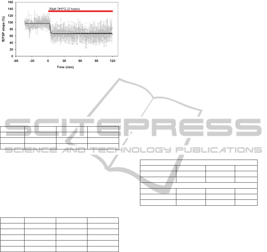
Figure 2: Measured mean LTD response curve +/-std
(gray) with corresponding best first order model (dashed)
and best second order model (black) (2 hours application
of 30 M DHPG).
Table 1: Best first order model for mean LTD responses:
parameters a
1
, b
0
with corresponding standard errors, SE,
YIC, AIC, R
T
2
and time constant (TC).
a
1
SE(a
1
) a
2
SE(a
2
)
-0.6299 0.0683 -0.3733 0.0684
YIC AIC R
T
2
TC
-5.352 -13.357 0.90 65 s
Secondly, we identified different higher models.
The best third, fourth and fifth order models were
excluded because of over-parameterisation. The best
higher order model was a second order model with n
= m = 2 (see Table 2).
Table 2: Best second order model for mean LTD
responses: parameters a
1
, a
2
, b
0
, b, with corresponding
standard errors, SE, YIC, AIC and R
T
2
.
a
1
SE(a
1
) a
2
SE(a
2
)
-1.6023 0.0661 0.6037 0.0644
b
0
SE(b
0
) b
1
SE(b
1
)
-0.3957 0.0636 0.3944 0.0655
YIC AIC R
T
2
-5.075 -20.824 0.89
For this model, the R
T
2
value was 0.89 and the fit
was similar to the one of the first order model (see
Figure 2). One pole was close to unity, indicating an
integrator effect. In addition, the sum of the
numerator parameters of the second order TF model
was almost equal to zero (b
0
+ b
1
= -0.0013; see
Table 2), which could imply a switch-like effect of
the DHPG input on the synaptic efficacy (cf. k=0 in
Figure 2). This effect can be shown starting from
x(k), the noise free output of the general TF model
equation:
( ) 1.602 ( 1) 0.604 ( 2)
0.396 ( ) 0.394 ( 1)
xk xk xk
uk uk
(7)
The synapses react especially at the start of the drug
application for which u(k)
u(k-1) (e.g. for k=0 in
Figure 2). When the applied drug concentration is
steady, the effect of the drug will saturate and there
will be a neglible effect on the synaptic outputs
since 0,396u(k)
0,394u(k-1) for u(k) = u(k-1).
3.2 Model-based Identification of
Dominant Sub-processes
The accurate second order model suggested that
there are two coupled dominant processes which
underlie mGluR-LTD. From a mathematical point of
view, two possible configurations of first order
models were suggested: a parallel circuit and a
feedback circuit (see Figure 1). The serial
configuration was mathematically impossible for
this model structure (n = m = 2; see Table 2) and
could be excluded. The model characteristics of the
first order models for the feedback and parallel
solution are shown in Table 3.
Table 3: First order models, TF1 and TF2, obtained after
decomposing the second order model for parallel and
feedback configuration (see Figure 1 and 2).
TF1
Configuration a
1
b
0
TC
Parallel -0.9965 0.0002 24 hrs
Feedback -0.6058 -0.3958 60 s
TF2
Configuration a
1
b
0
TC
Parallel -0.6058 -0.3959 60 s
Feedback -0.9967 -0.0006 25 hrs
4 DISCUSSION
Recent advances of imaging techniques have made
possible to visualise and quantify synaptic changes
on a time scale of months or years. These studies
have shown that synapses have many dynamic
properties that appear (and disappear) repeatedly
over time (Hou et al., 2006); (Kondo and Okabe,
2011). Therefore, dynamical analyses of synaptic
plasticity can highly contribute to fully comprehend
the underlying synaptic mechanisms. In many
studies, electrophysiological brain slice recordings
are used to measure the synaptic strength and to
analyse the different forms of synaptic plasticity.
However, in most studies the fEPSP recordings are
only statically analysed and the fEPSP slopes are
compared for only one time point or a limited
number of time points after the induction of LTD or
LTP. To the authors’ knowledge, it is the first time
that fEPSP slopes of mGluR-LTD responses are
dynamically described using TF models.
DynamicData-basedModellingofSynapticPlasticity:mGluR-dependentLong-termDepression
51

The second order model could be decomposed
into two first order models and suggest that two
major sub-processes underlie mGluRLTD: one slow
and one fast sub-process (see Table 3). A parallel
circuit and a feedback circuit were suggested as
candidate configurations of these two sub-processes.
Possibly, the fast time constants describes the
fast processes immediately after induction mediated
by activation of the ERK/MAPK pathway and
tyrosine dephosphorylation (e.g. of GluR2) with the
tyrosine phosphatase striatal-enriched tyrosine
phosphatase (STEP) as a main player.
The slow time constant, in contrast, is likely to
reflect structural changes, for example in spine
number and morphology, that were demonstrated in
other models of synaptic plasticity to be protein-
synthesis-dependent and to occur on a time-scale of
hours (Fukazawa et al., 2003; Raymond, 2007).
Many studies show the presence of feedback loops
in cellular control systems (Mitrophanov &
Groisman, 2008). Neural mechanisms are known to
contain many non-linearities, but our modelling
results confirm other studies in which discrete-time
linear system identification techniques were
succesfully used for modelling brain signals (e.g.
Liu et al., 2003; Westwick et al., 2006; Behrend et
al., 2009).
5 CONCLUSIONS
Discrete-time TF models are interesting to
investigate mGlu receptor-dependent LTD, because
of their computational and conceptional simplicity
and since they are able to combine the advantages of
a data-based approach (accurate models) with a
mechanistic approach (meaningful parameters). This
study suggests that the dynamic data-based
modelling approach can be a valuable tool for
reverse engineering of mGluR-dependent LTD
responses. Moreover, this approach can also be
extended to other forms of LTD and LTP using
other induction protocols as input for the TF models.
It is expected that such system identification
methods can aid to unravel the complexities of
synaptic function and its role in disease.
REFERENCES
Akaike, H. (1974). A new look at the statistical model
identification. IEEE Transactions on Automatic
Control, 19, 716–723.
Balschun, D., Wolfer, D.P., Gass, P., Mantamadiotis, T.,
Welzl, H., Schutz, G., Frey, J. U., & Lipp, H. P.
(2003). Does cAMP response element-binding protein
have a pivotal role in hippocampal synaptic plasticity
and hippocampus-dependent memory? Journal of
Neuroscience, 23, 6304-6314.
Behrend, C.E., Cassem, S.M., Pallone, M.J.,
Daubenspeck, J.A., Hartov, A., Roberts, D.W., &
Leiter J.C. (2009). Toward feedback controlled deep
brain stimulation: dynamics by metabotropic
glutamate receptors. Journal of Neuroscience
Methods, 23, 6304-6314.
Bellone, C., Lüscher, C., & Mameli, M. (2008).
Mechanisms of synaptic depression triggered by
metabotropic glutamate receptors. Cellular and
Molecular Life Sciences, 65, 2913–23.
Collingridge, G. L., Peineau, S., Howland J. G., & Wang
Y. T. (2010). Long-term depression in the CNS.
Nature Reviews Neuroscience, 11, 459–73.
Fukazawa, Y., Saitoh, Y., Ozawa, F., Ohta, Y., Mizuno,
K., & Inokuchi, K. (2003). Hippocampal LTP is
accompanied by enhanced F-actin content within the
dendritic spine that is essential for late LTP
maintenance in vivo. Neuron, 38, 447–460.
Hou, L., Antion, M.D., Hu, D., Spencer, C.M., Paylor, R.,
& Klan, E. (2006). Dynamic translational and
proteasomal regulation of fragile X mental retardation
protein controls mGluR-dependent long-term
depression. Neuron, 51, 441–454.
Izhikevich, E.M. (2007). Dynamical systems in
Neuroscience. MIT press, Cambridge
Jarvis, A.J., Stauch, V.J., Schulz, K., & Young, P.C.
(2004). The seasonal temperature dependency of
photosynthesis and respiration in two deciduous
forests. Global Change Biology, 10, 939–950.
Kandel, E.R. (2001). The molecular biology of memory
storage: a dialogue between genes and synapses.
Science, 294, 1030–1038.
Kondo, S., & Okabe, S. (2011). Turnover of Synapse and
Dynamic Nature of Synaptic Molecules In Vitro and
In Vivo. Acta Histochem Cytochem, 44, 9–15.
Liu, Y., Birch, A.A., & Allen, R. (2003), Dynamic
cerebral autoregulation assessment using an ARX
model: comparative study using step response and
phase shift analysis. Cell and Tissue Research, 25,
647-653.
Ljung, L. (1987). System identification: theory for the
user. Prentice-Hall, Englewood Cliffs, N.J.,
Lüscher, C., & Huber, K. (2010). Group 1 mGluR-
Dependent Synaptic Long-Term Depression:
Mechanisms and Implications for Circuitry and
Disease. Neuron, 65, 445–459.
Malenka, R.C., & Bear, M.F. (2004). LTP and LTD: an
embarrassment of riches. Neuron, 44, 5–21.
Manninen, T., Hituri, K., Kotaleski, J. H., Blackwell, K.
T., & Linne, M.-L. (2010). Postsynaptic Signal
Transduction Models for Long-Term Potentiation and
Depression. Frontiers in Computational Neuroscience,
4, 152.
Massey, P. V., & Bashir, Z. I. (2007). Long-term
depression: multiple forms and implications for brain
BIOSIGNALS2013-InternationalConferenceonBio-inspiredSystemsandSignalProcessing
52

function. Trends in Neurosciences, 30, 176–184.
Mitrophanov, A.Y., & Groisman, E.A. (2008). Positive
feedback in cellular control systems. Bioessays, 30,
542–555.
Neves, G., Cooke, S.F., & Bliss T.V.P. (2008). Synaptic
plasticity, memory and the hippocampus: a neural
network approach to causality. Nature Reviews
Neuroscience, 9, 65–75.
Nieus, T., Sola, E., Mapelli, J.,Saftenku, E., Rossi, P., &
D’Angelo, E. (2006). LTP regulates burst initiation
and frequency at mossy fiber-granule cell synapses of
rat cerebellum: experimental observations and
theoretical predictions. Journal of Neurophysiology,
95, 686–699.
Raymond, C.R. (2007). LTP forms 1, 2 and 3: different
mechanisms for the ”long” in long-term potentiation.
Trends in Neurosciences, 30, 167–175.
Richter, J.D., & Klann, E. (2009). Making synaptic
plasticity and memory last: mechanisms of
translational regulation. Genes & Development, 23, 1–
11.
Shouval, H.Z., Bear, M.F., & Cooper, L.N. (2002). A
unified model of NMDA receptordependent
bidirectional synaptic plasticity. Proceedings of the
National Academy of Sciences of the United States of
America, 99, 10831–10836.
Tambuyzer, T., Ahmed, T., Berckmans, D., Balschun, D.,
& Aerts, J. (2011). Reverse engineering of
metabotropic glutamate receptor-dependent long-term
depression in the hippocampus. BMC Neuroscience
2011, 12(Suppl 1): P1.
Taylor C.J., Pedregal, D. J., Young, P. C., &W. Tych.
(2007). Environmental time series analysis and
forecasting with the CAPTAIN toolbox.
Environmental Modelling & Software, 22, 797–814.
(http://www.es.lancs.ac.uk/cres/captain/)
Tomlin, C.J., & Axelrod, J.D. (2005). Understanding
biology by reverse engineering the control.
Proceedings of the National Academy of Sciences of
the United States of America, 102, 4219–4220.
Westwick, D.T., Pohlmeyer, E.A., Solla, S.A., Miller,
L.E., & Perreault, E.J. (2006). Identification of
multiple-input systems with highly coupled inputs:
application to EMG prediction from multiple
intracortical electrodes. Neural Computation, 18, 329-
55.
Young, P.C. (1984). Recursive estimation and time series
analysis. Springer-Verlag, Berlin.
DynamicData-basedModellingofSynapticPlasticity:mGluR-dependentLong-termDepression
53
