
Disjunctive Normal Form of Weak Classifiers for Online Learning
based Object Tracking
Zhu Teng and Dong-Joong Kang
Institute of Mechanical Engineering, Pusan National University
Busandaehak-ro 63beon-gil Geumjeong-gu, Busan, South Korea
Keywords: DNF of Weak Classifiers, Object Tracking, Online Learning.
Abstract: The use of a strong classifier that is combined by an ensemble of weak classifiers has been prevalent in
tracking, classification etc. In the conventional ensemble tracking, one weak classifier selects a 1D feature,
and the strong classifier is combined by a number of 1D weak classifiers. In this paper, we present a novel
tracking algorithm where weak classifiers are 2D disjunctive normal form (DNF) of these 1D weak
classifiers. The final strong classifier is then a linear combination of weak classifiers and 2D DNF cell
classifiers. We treat tracking as a binary classification problem, and one full DNF can express any particular
Boolean function; therefore 2D DNF classifiers have the capacity to represent more complex distributions
than original weak classifiers. This can strengthen any original weak classifier. We implement the algorithm
and run the experiments on several video sequences.
1 INTRODUCTION
Interest in motion analysis has recently increased in
tandem with the development of enhanced motion
analysis methodology and processing capabilities.
Tracking entails following the motion of a smaller
set of interest points or objects in video sequences,
and is accordingly one of the most significant
categories of motion analysis. Many applications of
tracking (Avidan, 2004, Stauffer, 2000, etc.),
including human face tracking, pedestrian tracking,
and vehicle tracking, have been developed in
accordance with the widespread use of surveillance.
Taking tracking as a binary classification problem
was first addressed in the mean-shift algorithm of
(Comanciu, 2003), which trains a classifier to
differentiate an object from the background. As
encouraging results have been obtained (Parag, 2008,
Tieu, 2000, Kalal, 2010, etc.), this approach has
come into wide use. The classifier can be trained
offline or online. The difference between offline
learning and online learning is that offline learning
requires the entire training set to be available at
once, and sometimes it requires random access to the
data, while online learning only involves one pass
through the training data (Oza, 2001). Furthermore,
offline learning methods have limited adaptability to
variation of the objects. (Oza, 2001) and (Freund,
1995) present both the theoretical and experimental
evidence that online boosting can achieve
comparable performance to its offline counterparts.
Our work concentrates on online boosting.
Online boosting has been studied by many
researchers, and it is the most successful ensemble
learning method. Shai Avidan proposed ensemble
tracking, which combines a collection of weak
classifiers into a single strong classifier, and treats
tracking as a binary classification problem. A feature
selection framework based on online boosting is
introduced in (Grabner, 2006). An online semi-
supervised boosting has been presented in (Grabner,
2008); it ameliorates the drifting problem in tracking
applications by combining the decision of a given
prior and an on-line classifier. (Stalder et al., 2009)
further amalgamated a detector, recognizer, and
tracker to track various objects. (Danielsson et al.,
2011) used two derived weak classifiers to suppress
combinations of weak classifiers whose outputs are
anti-correlated on the target class. If a drifting
problem occurs, it suggests that the error, which may
be magnified, results in an incorrect decision of the
object in object tracking, i.e., adapting to other
objects. Though an error accumulation can also lead
to a drifting problem, the fundamental reason for
drifting is the erroneous estimation of the object,
138
Teng Z. and Kang D..
Disjunctive Normal Form of Weak Classifiers for Online Learning based Object Tracking.
DOI: 10.5220/0004240501380146
In Proceedings of the International Conference on Computer Vision Theory and Applications (VISAPP-2013), pages 138-146
ISBN: 978-989-8565-48-8
Copyright
c
2013 SCITEPRESS (Science and Technology Publications, Lda.)

which is determined by the classifier when tracking
is considered as a binary classification problem.
In this paper, we propose a 2D disjunctive
normal form (DNF) of weak classifiers. The
conventional weak classifier uses linear classifiers or
stumps, which label samples just better than random
guessing. Generally, this classifier takes the form of
a threshold. A sample is tagged to an object category
when the feature of the sample is larger or lower
than the threshold. This conventional weak classifier
is termed 1D weak classifier in our paper. The input
data of the 2D DNF of weak classifiers are
constituted by all the pairwise combinations of data
utilized by all the 1D weak classifiers, and thus this
approach is more accurate. As one full DNF can
represent any particular Boolean function, the 2D
DNF can express more difficult distributions than
the conventional weak classifiers, and it also can be
employed on top of any original weak classifier. To
resolve the drifting problem, we combine it with a
reset mechanism. On the one hand, the DNF can
substantially decrease the error rate, which is the
fundamental cause of drifting, and on the other hand,
the reset mechanism suppresses error accumulation.
The contributions of this paper include: (i) the
formulation of a novel type (DNF) of weak
classifiers, and (ii) diversified features used in the
tracking system, which is implemented by analyzing
manifold features in the feature pool from the first
frame of the video and determines the most
appropriate features.
The reminder of this paper is organized as
follows: Section 2 provides a brief introduction of
AdaBoost. DNF tracking is illustrated in Section 3,
along with definitions and applications of DNF
classifiers. Section 4 presents the experiments and
conclusions follow in Section 5.
2 ADABOOST AND ENSEMBLE
TRACKING
To explain the basic notation, we will first briefly
review AdaBoost (Freund, 1995). A strong classifier
of AdaBoost is implemented by combining a set of
weak classifiers. Many tracking algorithms are
developed based on AdaBoost (Avidan, 2005).
Generally, the algorithm is based on pixels, and the
strong classifier determines if a pixel belongs to the
object or not. It employs the addition and removal of
weak classifiers to adapt to variation of the object
appearance or background. The weak classifier used
in (Avidan, 2005) is a linear classifier in a least-
squares manner or other classifiers (such as stumps,
perceptrons). Each pixel is represented by an 11D
feature vector, which is created by a combination of
the local orientation histogram and pixel colors. This
feature vector can be computed easily, and is
appropriate for object detection tasks (Levi, 2004).
Weak classifier:
Let
N
ii
y
1i
},{
=
x
denote N examples and their
labels, respectively, and
11
i
R∈x
and
}1,1{
+
−
∈
i
y
;
the weak classifier can then be represented by
],1[},1,1{:)(
11
TtRh
t
∈+−→x
(1)
where T is the number of weak classifiers.
Strong Classifier:
The strong classifier is defined as a linear
combination of a collection of weak classifiers. It is
given by sign(H(x)) and
∑
=
=
T
t
tt
hH
1
)()( xx
α
(2)
t
t
t
err
err−
=
1
log
2
1
α
(3)
∑
=
−=
N
i
itit
yhwerr
1
i
|)(| x
(4)
where w
i
is the weight of the i
th
example, and
weights are updated in the process of training weak
classifiers (Eq. (5)).
|))(|(
i itt
yh
ii
eww
−
=
x
α
(5)
3 DNF TRACKING
In this session, we propose a novel tracking method
that is based on the 2D DNF classifier. Session 3.1
describes the motivation for using the 2D DNF
classifier rather than the 1D weak classifier in
tracking, and defines the 2D DNF classifier.
Procedures for tracking based on 2D DNF classifiers
are illustrated in Session 3.2.
3.1 DNF Classifier
The proposed 2D DNF classifier is first motivated
by the drifting problem in ensemble tracking. The
drifting problem entails two important aspects: the
fundamental cause of drifting is the misclassification
DisjunctiveNormalFormofWeakClassifiersforOnlineLearningbasedObjectTracking
139
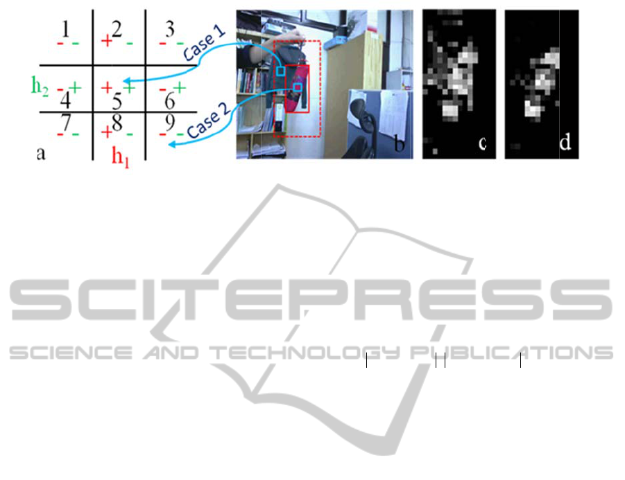
Figure 1
:
Confiden
c
rate of
w
action i
f
strong
c
classifie
r
linear c
o
Tak
e
Daniels
s
classifie
r
feature
s
shown i
n
suggests
p
ositive
negative
We des
c
sign of
c
1 the str
o
p
atch co
r
p
atch c
a
see that
(such a
s
classifie
d
combin
a
classifie
r
2D
D
Let
{
their la
b
should
b
is the n
u
feature
d
employ
e
quantifi
e
i
ij
≤ ,1,b
defined
a
:
Stimulus ex
a
ce map of the
s
w
eak classifie
r
f
drifting take
s
c
lassifier is
a
r
s, there are
o
mbinations c
a
e
a 2D feat
u
s
on, 2011).
A
r
s, h
1
(x) an
d
s
pace into p
o
n
Fig. 1 (a).
that classi
fi
region, and
a
region that
c
ribe the gre
e
c
lassifier h
2
(x
)
o
ng classifier
r
rectly (alwa
y
a
nnot be corr
e
some regio
n
s
region 5),
a
d
as ‘-’ (s
u
a
tion of we
a
r
) cannot ove
r
D
NF cell clas
s
},
{
f
yp
denot
e
b
els, respecti
v
b
e the value -
1
u
mber of exa
m
d
ata tha
t
w
e
e
d in classifi
c
e
d into
m
mj ≤
. The
a
s:
:)(
f2
R
h
Dcf
p
a
mple. (a) 2D
s
econd frame (
c
r
s, and the ot
h
s
place. Eve
n
a
linear com
b
still many
a
nnot present
.
u
re space as
A
ssume ther
e
d
h
2
(x), eac
h
o
sitive and n
e
A region wi
t
fi
er h
1
(x) ca
t
a
red minus
is labelled
by
e
n plus sign
)
similarly. A
cannot classi
f
y
s ‘+’), and i
n
e
ctly labelled
n
s are always
a
nd some re
g
u
ch as regio
n
a
k classifiers
r
come this pr
o
s
ifier:
e
examples o
v
ely, where e
a
1
or +1,
=
f
p
m
ples, and
d
e
ak classifie
r
s
c
ation. The
p
m
m
×
b
ins,
2D DNF
}1,1{
2
+−→
R
feature space.
c
) and the fifth
f
h
er is the rem
e
n
though the
f
b
ination of
w
distributions
an example
e
are two
w
h
classifying
e
gative regio
n
h
a red
p
lus
t
egorizes it
a
sign stands
f
y
classifier h
and green
m
s
a resul
t
, in
C
f
y the backgr
o
Case 2 the o
b
(always ‘-’).
classified a
s
g
ions are al
w
n
9). The li
(or the st
r
o
blem.
f
the f
th
cell
a
ch element
o
N
hh
ji
×
=
2
];[ dd
i
h
and
j
h
d ar
e
s
h
i
and h
j
h
p
lane
i
h
d
d −
denoted
cell classifie
(b) The first
f
rame (d).
e
dial
f
inal
w
ea
k
that
(O.
w
eak
the
n
s as
sign
a
s a
f
or a
1
(x).
m
inus
C
ase
o
und
b
ject
We
s
‘+’
w
ays
i
near
r
ong
and
o
f
y
N
, N
e
the
h
ave
j
h
d
is
b
y
e
r is
(6)
ma
p
C
b
C
b
ex
a
oth
e
all
ne
g
cla
s
uni
o
im
a
20
0
tot
a
lar
g
obj
e
trai
cla
s
ha
v
cla
s
p
ix
e
obj
e
co
m
the
M.
frame with t
h
For each col
p
ping relatio
n
=h
fiDcf
)(
2
p
,{ |
,
ij k fk ij
ij
by b
b
⎧
∈∧
⎪
=
⎨
∅
⎪
⎩
p
|.| indicates
t
ij
b
represents
t
a
mples than
t
e
rwise it is a
bins that ha
v
g
ative examp
s
sified as
p
os
i
o
n.
As a simple
e
a
ge as a 1D
0
4) related to
a
l number o
f
g
er than that
i
e
ct might b
e
n
ing by 1
D
s
sifier). If th
e
v
e the same
E
s
sifier can d
i
e
ls of the obj
e
ct.
2D DNF cla
s
The 2D DN
m
bination of
a
number of 2
D
h
e object in t
h
u
mn vector
p
n
ship is prese
n
⎪
⎩
⎪
⎨
⎧
−
∈
≤
oth
e
fi
,1
,1
1
p
1} { |
kkfkij
yyb
otherwise
∧
=> ∈p
t
he cardinalit
y
t
he bin
ij
b
if
t
t
he negative
null set.
ji
≤
≤ ,1
U
v
e more posit
i
l
es in each
i
tive if it ent
e
e
xample, con
f
eature and
1
edge as ano
t
f
red pixels
i
n the object,
e
recognized
D
feature o
f
e
red pixels
o
E
OH feature
fferentiate th
e
ct are possi
b
s
sifier:
F
classifier
i
a
set of 2D D
N
D
DNF cell c
l
h
e solid red r
e
fi
p
in
f
p
, th
e
n
ted in Eq. (7
)
≤
≤
e
rwise
Cb
ij
mji,
U
1} , [1, ]
j
k
ykN∧=− ∈
y
of a set i
n
t
here are mor
e
examples in
ij
m
Cb
≤
is th
e
t
ive example
s
bin. An e
x
e
rs into any
b
n
sider R chan
n
1
D of EOH
(
t
her 1D feat
u
in the back
g
then red pix
as backgro
u
f R chann
e
of backgrou
n
as the objec
t
h
em, and the
n
b
le to be reco
i
s defined a
s
N
F cell class
i
l
assifiers is d
e
e
ctangular.
e
specific
)
.
(7)
(8)
n
Eq. (8).
e
positive
that bin,
e
union of
than the
ample is
b
in of this
n
el of the
(
Levi, K.,
u
re. If the
g
round is
e
ls in the
u
nd when
e
l (weak
n
d do not
t
, 2D cell
n
the red
g
nized as
a linear
i
fiers, and
e
noted by
VISAPP2013-InternationalConferenceonComputerVisionTheoryandApplications
140

∑
=
=
M
f
fDcfDfD
hH
1
222
)()( px
α
(9)
Let
},...,,{
w21
ddd=S
be the set of feature data
that weak classifiers have used; then
}
f
{p
is a set of
all the pairwise combinations of the set S, that is,
f
p
is a subset of two distinct elements of S (as shown in
Eq. (10)).
},{}{
ji
,,1
f
ddp
jiwji <≤≤
= U
(10)
w is the row number of feature data that weak
classifiers have employed in Eq. (10), and it is no
larger than the dimension of the feature space.
3.2 2D DNF Classifiers for Tracking
To start tracking, feature data are first extracted.
Diverse kinds of features are obtained from the first
frame of the video sequence, and they are employed
to train the new weak and DNF cell classifiers. The
best kind of feature according to the performance of
these features on the first frame is then selected by
the feature pre-selector. Classifiers are trained in
initialization, and are constantly updated in the
following frames. We use an ensemble of weak and
DNF classifiers to determine whether a patch
belongs to the object or not, and a confidence map is
also constructed during this process. The peak of the
map, which is achieved by the integral image (P.
Viola, 2001) of the confidence map, is believed to be
the new object position. The feature data of the new
position of the object are used to update classifiers.
3.2.1 Feature Pre-selector
In order to track different objects, the most suitable
features to employ are not always the same, and
feature selection techniques have been researched by
many researchers (see Ref (R. Collins, 2005) as an
example). In order to apply the most appropriate
features in diversified tracking missions, the feature
pre-selector is constituted. It is a product of the
compromise of the amount of computation and the
adaptability of different objects to be tracked. All
kinds of the features are calculated from the first
frame of the video sequence. Features of a fixed
number of patches used for learning are randomly
selected, and the performance of classifiers for each
kind of feature is assessed on other randomly
selected patches for the first frame. The feature pre-
selector chooses the feature with the best
performance. After the type of feature is determined,
the remaining frames will only calculate this kind of
feature. Therefore, the time required for calculating
features is reduced as only the pre-selected feature is
employed once tracking has commenced. The
features used in this work include the local binary
pattern (LBP) (T. Ahonen, 2004), Haar feature (P.
Viola, 2001, Papageorgiou, 1998), and local edge
orientation histograms (EOH) (Levi, K., 2004). All
these features are extracted based on patches and are
combined with the average R, G, and B values in
each channel of the patches.
3.2.2 Outlier Elimination
Outliers in our work are defined as patches in the
bounding box of the object but do not belong to the
object. Outliers can affect weak and DNF classifiers
in the processes of training and updating.
In the initialization step when training classifiers,
even though the object is given by a bounding box,
patches in this bounding box do not always belong
to the object to be tracked, because the object is not
always a shape of rectangle. This kind of outliers is
represented as minority points in the bins of feature
space because outliers are minority compared to the
majority features of the object in the bounding box.
To apply it to our work, Eq. (8) is changed to Eq.
(11) in the real implementation as shown below. The
parameter r should be a positive integer (we set it to
5 in our experiments).
{| 1}{| 1},[1,]
ij kfkij k kfkij k
ij
by by y by rk N
Cb
otherwise
⎧
∈∧ =− ∈∧ =−> ∈
⎪
=
⎨
∅
⎪
⎩
pp
(11)
We first attempted to use the labeled data in the
last frame to update classifiers, i.e. semi-supervised
learning, which lends adaptability to the system;
however, if mistakenly estimated data are used, the
system can easily drift. In other words, when
classifiers are updated, patches in the bounding box
are labelled as positive example (Eq. 12,
i
pa
represents the i
th
patch), whereas in fact they should
be labeled as negative examples.
⎪
⎩
⎪
⎨
⎧
−
+
=
otherwise
rectangleobjecttheinispa
y
i
i
1
1
(12)
If we do not reject these patches, they will be
trained as the object, which may lead to drifting.
Employing it in our algorithm, patches in the
bounding box that have a relatively larger
confidence can be labelled as positive (Eq. (13)).
DisjunctiveNormalFormofWeakClassifiersforOnlineLearningbasedObjectTracking
141

1( (
1
ii
i
p
a object rectangle) conf(pa ) 0.5)
y
otherwise
+∈ ∧ >
⎧
=
⎨
−
⎩
(13)
3.2.3 Specific DNF Algorithm of Tracking
Algorithm 1: DNF algorithm for tracking
Input: a video sequence with n frames;
a bounding box for the object in the first
frame.
Output: a bounding box of the object for the
remaining frames.
Initialization (for the First Frame):
(1) Extract all types of features from the first frame
]},1[,,{
ff
Ff ∈yx
, where F is the total number of
types of features. The number of positive and
negative patches used for training is fixed, and these
patches are randomly selected.
(2) Train weak classifiers and 2D DNF classifiers
for each type of feature. Randomly select patches
from the first frame, extract features of these patches
as test examples, and the feature with the minimum
error is chosen for use in the following frame.
(3) Set the state of tracking as FOUND, and save
initial classifiers and data.
For a New Frame:
(1) Draw the pre-selected feature of all the patches
from the background of the current frame.
Generally, the background is defined as twice the
size of the object, while the detected region is spread
to the whole frame in the case of losing the object.
(2) Examine all the patches with the combination of
weak classifiers and 2D DNF cell classifiers
∑∑
==
+=
M
f
fDcfDf
T
t
tt
hhH
1
22
1
)()()( pxx
αα
, and the
confidence map is created.
∑∑
==
+=
M
f
fDcfDf
T
t
tt
hhconfidence
1
22
1
)()( px
αα
(3) Obtain the object position and the current
confidence from the integral image of the confidence
map. If the current confidence is not larger than a
threshold TH1, the state of tracking is determined as
LOST. The classifiers are restored to their initial
states, and the detected region is spread to the whole
frame.
(4) If the current frame is under the LOST state and
the current confidence is larger than a threshold
TH2, the state of tracking is reinstated to the
FOUND state.
(5) If the current frame is under the FOUND state,
update classifiers.
In the update step, the positive data for updating
are comprised of the labeled data from the last frame
and the initial positive data. The updating of weak
classifiers is the same with (Avidan, 2005), and as
the weak classifiers update, the data for the DNF
classifiers are updated and the DNF classifiers are
renovated.
4 EXPERIMENTS
In this section, we implement the proposed
algorithm in Matlab, evaluate it on several video
sequences, and compare its performance with that of
three other tracking methods. We also use sequences
of PROST dataset and the evaluation method
provided by (Santner, 2010) to demonstrate the
performance of our algorithm. Furthermore, the
performance of the DNF cell classifier is weighed
against that of a weak classifier in Section 4.1, the
performance comparison of DNF classifier and
strong classifier is presented in Section 4.2, and the
effects of exclusion of outliers are illustrated in
Section 4.3. All of the experiments are executed on
an Intel(R) i5 2.80GHz desktop computer.
4.1 2D DNF Cell Classifier VS Weak
Classifier
This experiment is carried out to evaluate the
performance of the DNF cell classifier, the
performance of which is also compared with that of
weak classifiers (Avidan, 2005). The data used in
this experiment are the 9
th
dimension and 10
th
dimension data of EOH feature and are normalized
to the range [0, 1]. The feature is calculated based
on patches, the radius of which is set to 5. Classifiers
are trained on the first frame of the video sequence
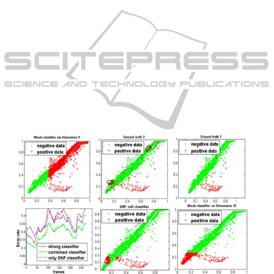
and updated in the following frames; Fig. 2 shows
the results of the fifth frame. Features of all the
patches in the fifth frame are extracted. Classifiers
are then applied to these features and the patches are
classified to the object category or background
category. Each point in Fig. 2 represents a patch in
the image, where a red plus sign indicates an object
patch and a green point denotes a background patch.
We show two situations of the ground truth. Only
object patches are set to positive data (Fig. 2 (a)) for
the first situation, that is, with ideal outliers
excluded. For the other situation, patches in the
bounding box are all put to the positive data set (as
shown in Fig. 2 (b)). It is obvious that the red plus
signs in the black ellipses of Fig. 2 (b) are outliers.
For instance, patches of the background coat (green
VISAPP2013-InternationalConferenceonComputerVisionTheoryandApplications
142
color) in the solid red rectangle (object bounding
box) in Fig. 1 (b) are this kind of outlier. We can see
that the performance of the DNF cell classifier (Fig.
2 (e)) is much better than that of weak classifiers
(Figs. 2 (c, d)) even though it is slightly influenced
by the outliers in the object bounding box. If the
performance of the cell classifiers is good, we can
expect the final DNF classifier will be better.
4.2 2d DNF Classifier Vs Strong
Classifier
Fig. 2 (f) shows the error rates of three classifiers to
demonstrate to what extent 2D DNF classifier can
improve the performance, compared with the strong
classifier. As the experiment is to compare the
classification capability of these three classifiers, no
updates or other techniques are used (such as outlier
elimination). We train the three classifiers on the
first frame, and test on more than 260 other frames
(the video sequence used here is “car”, see also Fig.
3 (a)). For each frame, features of all the patches are
calculated (EOH feature is employed), and the error
rate is defined as the number of correctly classified
patches divided by the whole number of patches.
Furthermore, we add the only-DNF classifier, which
is only a linear combination of DNF cell classifiers.
The combined classifier in the Fig. 2 (f) is the
classifier used in Algorithm 1, which is a linear
combination of weak classifiers and 2D DNF cell
classifiers. It is clear that the combined classifier has
the best classification capability compared to the
other two classifiers.
4.3 Outlier Elimination Experiment
The goal of this experiment is to view the effects of
outlier elimination (shown in Fig. 1). In the
initialization step, positive training data that are
obtained from the object bounding box of the first
frame (Fig. 1(b)) include data that do not belong to
the object, and if these data are not rejected in the
updating process, the outliers will be trained in the
same manner as the object, which leads to the
drifting of the tracker. In each bin of feature space,
there are more patches from the object than from
outliers, even though these outliers are labelled as
the object, many of them cannot win over the object
data (Eq. (11)). Furthermore, most of the winning
outliers can be restrained in the updating procedure,
as patches with lower confidence are not updated to
the next frame. As shown in Fig. 1(c), patches from
the green coat in the background are initially trained
as the object, but are soon restricted in the following
frames (Fig. 1(d)) as the outlier exclusion takes
effect.
Figure 2: Experiments for comparisons of weak classifiers and DNF cell classifiers. a) Ground truth with only patches from
the object set as positive data; b) Ground truth with patches in the object bounding box set as positive data; c) classifying
results of weak classifier 1; d) classifying results of weak classifier 2; e) classifying results of DNF cell classifier; f)
comparative results of strong classifier and DNF classifier.
d
e
f
a
b
c
DisjunctiveNormalFormofWeakClassifiersforOnlineLearningbasedObjectTracking
143
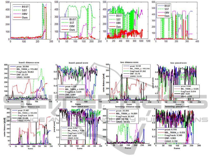
Figure 3:
case, c)
p
Figure 4:
Distance
4.4
E
The
p
r
o
objects.
source c
o
http://w
w
.htm) a
r
several
v
are BSS
T
2008), a
n
all the v
i
p
rovide
d
box. Th
e
are sho
w
Euclide
a
b
oundin
g
of the g
r
p
osition
s
frame. P
The
road. Al
b
ut the
disappe
a
Center differe
n
edestrian, d) c
u
Comparative r
e
score: the mea
n
E
xperimen
t
o
posed algor
i
Our algorith
m
o
des of all th
e
w
w.vision.ee.
e
r
e executed
v
ideo seque
n
T
of (S. Stal
d
n
d OBV of (
H
ideo sequenc
e
d
in the first
f
e
tracking res
u
w
n in Fig. 3, t
h
a
n distance
g
box of the
r
ound truth
bo
s
of objects a
r
arts of the fra
first video s
e
l four metho
d
performance
s
a
red from the
n
ces (in pixels)
u
p setting as th
e
e
sults of DNF
a
n
center locatio
n
t
s on Vide
o
i
thm can tr
a
m
and three o
t
e
three metho
d
e
thz.ch/boost
i
to track dif
f
n
ces. The oth
d
e
r
, 2009), SS
H
. Grabne
r
,
2
e
s is 640*48
0
f
rame manua
l
u
lts of the fo
u
h
e vertical a
x
between th
e
detected obj
e
o
unding box.
r
e acquired
m
me shots are
s
e
quence is a
d
s tracked th
e
s
varied as
t
clip. BSST
between the g
r
e
tracking obje
c
a
nd other four
m
n
error in pixel
o
Sequence
s
a
ck a variet
y
her methods
(
d
s are availab
i
ngTrackers/i
n
f
erent object
s
er three met
h
T
of (H. Gra
b
2
006). The si
z
0
and the obj
e
l
ly by a
b
oun
d
r
video seque
n
x
is of which i
s
e
center of
e
ct and the c
e
The ground
t
m
anually fram
e
s
hown in Fig.
car running
o
e
car well at
f
t
he car grad
u
and SST los
t
r
ound truth and
c
t.
m
ethods in the
s. Pascal score
:
s
y
of
(
The
b
le at
n
dex
s in
h
ods
b
ne
r
,
z
e of
e
ct is
ding
n
ces
s
the
the
e
nte
r
t
ruth
m
e by
5.
o
n a
f
irst,
u
ally
t
the
obj
e
wa
s
p
la
c
me
t
dis
a
(a)
me
t
not
tru
t
cli
p
p
la
c
In
t
b
o
u
b
a
c
ma
k
5(2
of
t
wa
s
ex
p
fra
m
alt
e
los
i
go
o
the tracking r
e
v
ideo sequenc
e
:
calculated by
E
e
ct at the fra
m
s
included,
O
c
e as the obje
t
hod lost th
e
a
ppeared fro
m
we can see th
t
hod converg
e
detect the o
b
t
h, because f
i
p
. Meanwhile
c
e as object,
r
t
he second c
l
u
nding box
o
c
kground pix
e
k
es tracking
e)), especiall
y
t
he object
b
o
u
s
tracked in
p
erimen
t
, BS
S
m
e and was
n
e
rnated betw
e
i
ng the
p
ede
o
d performan
c
sults. From lef
t
e
s provided in
R
E
q.(14).
m
e where rou
g
O
BV mistak
e
c
t (see Fig. 5
e
object whe
n
m
the video
s
a
t the curves
o
e
to zero, as t
h
b
ject. It is t
h
n
ally the car
,
OBV mist
a
r
esulting in a
l
l
ip, a pencil
c
o
f the
p
encil
e
ls when it
i
easily drifte
y
in the case
u
nding box is
t
the third vi
d
S
T lost the o
b
n
ot able to re
e
en detectin
g
strian, and
O
c
e but detect
e
ft
to right: a) ca
r
R
ef (Jakob San
t
g
hly 90% of
t
e
nly detecte
d
(1e) and (1f)
)
e
n 50% of t
h
s
equence. Fr
o
o
f BSST, SS
T
h
ese three m
e
h
e same as t
h
disappeared
a
kenly tracke
d
l
arge center
d
c
ase was tra
c
l
case inclu
d
is lifted up,
e
d (as show
n
where the b
a
the same. A
p
d
eo sequenc
e
b
ject at abou
t
e
-track the ob
j
g
the pedes
t
O
BV initiall
y
e
d the wrong
r
, b) pencil
t
ne
r
, 2010).
t
he object
d
another
)
, and our
h
e object
o
m Fig. 3
T
, and our
e
thods did
h
e ground
from the
d
another
ifference.
c
ked. The
d
ed many
and this
n
in Fig.
a
ckground
p
edestrian
e
. In this
t
the 20
th
j
ect, SST
t
rian and
y
showed
object at
VISAPP2013-InternationalConferenceonComputerVisionTheoryandApplications
144
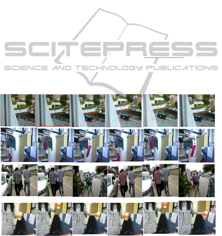
about the 700
th
frame (as shown in Fig. 5(3e) and
(3f)) and could not recover the detection of the
pedestrian thereafter (see Fig. 3(c)). Our method
provides a relatively good performance, but the
center difference is somewhat large (the other three
methods suffer the same problem). The reason for
this is that the pedestrian in this clip was sometimes
standing near the camera and appeared larger than
that in the initial frame but the size of the object
bounding box in our method is fixed during the
tracking process. The object of the fourth clip is a
cup. The cup disappeared twice in the video
sequence. The first disappearance was at about the
165
th
frame, and OBV lost the object from this frame
on (see Fig. 3(d)). In the case of the SST method, the
object was lost and recovered a number of times.
BSST provided relatively stable tracking but it failed
to track the object between two disappearances.
Adaptation to other objects occurred occasionally in
our method as well. However, this was remedied
quickly, which is manifested as sharp peaks in Fig.
3(d).
Besides these video sequences, we also testify
our method on the PROST dataset, the video
sequences in which were newly created by the
authors of (Jakob Santner, 2010) (The video
sequences and the code of the evaluation method are
available at
http://gpu4vision.icg.tugraz.at/index.php?content=su
bsites/prost/prost.php), and the two evaluation
methods shown in Fig. 4 are also provided by (Jakob
Santner, 2010). The first evaluation is the distance
score that represents the mean center location error
in pixels. The second evaluation method is PASCAL
score based on PASCAL challenge (M. Everingham,
2009). A frame is determined as a corrected tracked
frame if the overlap score of the frame proceeds 0.5.
The overlap score is calculated by Eq. (14), where
BB
D
denotes the detected bounding box and BB
GT
represents the ground truth bounding box. Each
point on the PASCAL score curve of Fig. 4 is the
overlap score for each frame, and the number in the
graph legend of PASCAL score figure represents a
percentage of correctly tracked frames for a
sequence.
)(
)(
GTD
GTD
BBBBarea
BBBBarea
score
∪
∩
=
(14)
The benchmarked methods of Fig. 4 involves the
Figure 5: Parts of frames of experimental results on video sequences. Processing methods: 1d-1f: SST, 2d-2f: BSST, 3d-3f:
OBV, 4d-4f: BSST, 1a-1c,2a-2c,3a-3c,4a-4c: our method.
4a #24
4b #166
4c #201
4d #24
4e #166
4f
#201
3a #28
3b #690
3c #719
3d #28
3e #690
3f #719
2a #54
2b #126
2c #185
2d #54
2e #126
2f #185
1e #241
1d #227
1a #227
1
b
#
241
1c #268
1f #168
DisjunctiveNormalFormofWeakClassifiersforOnlineLearningbasedObjectTracking
145

methods of PROST (Jakob Santner, 2010),
MIL_TR004_c (B. Babenko, 2009), FragTrack (A.
Adam, 2006), and GRAD (Klein, 2011). It shows
that our method achieves a best performance in
sequences of board and lemming, and a slightly less
good performance than PROST in sequences of
liquor and box. An average PASCAL score of our
method over the four sequences is 88.75%, which is
much better than the average of 80.375% for PROST
method.
5 CONCLUSIONS
This paper described a novel tracking method based
on a 2D DNF of weak classifiers. The data of the
DNF cell classifiers are constituted by pairwise
combinations of the data of weak classifiers, and
therefore the DNF can be utilized on top of any
weak classifiers. The image patch is determined to
belong to the object category or the background
category by an ensemble of weak classifiers and
DNF cell classifiers. The experiments demonstrate
that our method provides a good performance
compared to other methods but sometimes the center
difference is somewhat large due to the unvaried
object bounding box. For better tracking, we will
continue the present line of research with a scalable
object bounding box in the future.
ACKNOWLEDGEMENTS
This work was supported by the Basic Science
Research Program through the National Research
Foundation of Korea (NRF) funded by the Ministry
of Education, Science and Technology (No. 2009-
0090165, 2011-0017228).
REFERENCES
Avidan S., 2004. Support Vector Tracking. In IEEE Trans.
On Pattern Analysis and Machine Intelligence.
Stauffer, C. and E. Grimson, 2000. Learning Patterns of
Activity Using Real-Time Tracking. In PAMI,
22(8):747-757.
S. Avidan, 2005. Ensemble tracking. In Proc. CVPR,
volume 2, pages 494–501.
H. Grabner and H. Bischof, 2006. On-line boosting and
vision. In Proc. CVPR, volume 1, pages 260–267.
H. Grabner, C. Leistner, and H. Bischof, 2008. Semi-
supervised on-line boosting for robust tracking. In
Proc. ECCV.
S. Stalder, H. Grabner, and L. van Gool, 2009. Beyond
Semi-Supervised Tracking: Tracking Should Be as
Simple as Detection, But Not Simpler than
Recognition. In Proc. Workshop Online Learning in
Computer Vision.
O. Danielsson, B. Rasolzadeh, and S.Carlsson, 2011.
Gated Classifiers: Boosting under High Intra-Class
Variation. In Proc. CVPR.
N. Oza and S. Russell, 2001. Online bagging and boosting.
In Proc. Artificial Intelligence and Statistics, pages
105–112.
Freund, Y. Schapire, R. E, 1995. A decision-theoretic
generalization of on-line learning and an application to
boosting. In Computational Learning Theory:
Eurocolt 95, pp 23-37.
Comanciu, D., Visvanathan R., Meer. P, 2003. Kernel-
Based Object Tracking. In IEEE Trans. on Pattern
Analysis and Machine Intelligence (PAMI), 25:5, pp
564-575.
Levi, K., Weiss, Y, 2004. Learning Object Detection from
a Small Number of Examples: The Importance of
Good Features. In IEEE Conf. on Computer Vision
and Pattern Recognition.
P. Viola and M. Jones, 2001. Rapid object detection using
a boosted cascade of simple features. In Proc. CVPR,
volume I, pages 511–518.
Papageorgiou, Oren and Poggio, 1998. A general
framework for object detection. In International
Conference on Computer Vision.
T. Ahonen, A. Hadid, and M. Pietikäinen, 2004. Face
Recognition with Local Binary Patterns. In Proc.
Eighth European Conf. Computer Vision, pp. 469-481.
T. Parag, F. Porikli, and A. Elgammal, 2008. Boosting
adaptive linear weak classifiers for online learning and
tracking. In Proc. CVPR.
K. Tieu and P. Viola, 2000. Boosting image retrieval. In
Proc. CVPR, pages 228–235.
Z. Kalal, J. Matas, and K. Mikolajczyk, 2010. P-N
Learning: Bootstrapping Binary Classifiers by
Structural Constraints. In Proc. CVPR.
Jakob Santner, Christian Leistner, Amir Sa_ari, Thomas
Pock, and Horst Bischof, 2010. Prost: Parallel robust
online simple tracking. In Computer Vision and
Pattern Recognition (CVPR), 2010 IEEE Conference
on, pages 723-730, 13-18.
B. Babenko, M.-H. Yang, and S. Belongie, 2009. Visual
Tracking with Online Multiple Instance Learning. In
CVPR.
Klein, Cremers, 2011. Boosting Scalable Gradient
Features for Adaptive Real-Time Tracking. In Int.
Conf. on Robotics and Automation (ICRA).
A. Adam, E. Rivlin, and I. Shimshoni, 2006. Robust
fragments based tracking using the integral histogram.
In CVPR.
R. Collins, Y. Liu, and M. Leordeanu, 2005. Online
selection of discriminative tracking features. In PAMI,
27(10):1631–1643.
M. Everingham, L. Van Gool, C. K. I. Williams, J. Winn,
and A. Zisserman, 2009. The Pascal Visual Object
Classes (VOC) Challenge. In Int. J. Comput. Vision,
88(2):303–308.
VISAPP2013-InternationalConferenceonComputerVisionTheoryandApplications
146
