Collective Probabilistic Dynamical Modeling of Sleep Stage Transitions
Sergio A. Alvarez
1
and Carolina Ruiz
2
1
Department of Computer Science, Boston College, Chestnut Hill, MA 02467 U.S.A.
2
Department of Computer Science, Worcester Polytechnic Institute, Worcester, MA 01609 U.S.A.
Keywords:
Time Series, Clustering, Modeling, Markov, Data Mining, Sleep.
Abstract:
This paper presents a new algorithm for time series dynamical modeling using probabilistic state-transition
models, including Markov and semi-Markov chains and their variants with hidden states (HMM and HSMM).
This algorithm is evaluated over a mixture of Markov sources, and is applied to the study of human sleep stage
dynamics. The proposed technique iteratively groups data instances by dynamical similarity, while simultane-
ously inducing a state-transition model for each group. This simultaneous clustering and modeling approach
reduces model variance by selectively pooling the data available for model induction according to dynamical
characteristics. Our algorithm is thus well suited for applications such as sleep stage dynamics in which the
number of transition events within each individual data instance is very small. The use of semi-Markov models
within the proposed algorithm allows capturing non-exponential state durations that are observed in certain
sleep stages. Preliminary results obtained over a dataset of 875 human hypnograms are discussed.
1 INTRODUCTION
Sleep is divided into stages from all-night recordings
of physiological signals, particularly scalp EEG and
facial EOG (electro-oculography), following well-
established staging standards (Rechtschaffen and
Kales, 1968), (Iber et al., 2007). Stages span light
sleep (stages N1 / NREM1 and N2 / NREM2), deep
sleep (slow wave sleep, or SWS), and a stage tradi-
tionally associated with dreaming – Rapid Eye Move-
ment (REM) (dreams are known to occur during SWS
as well (Cavallero et al., 1992)). The temporal se-
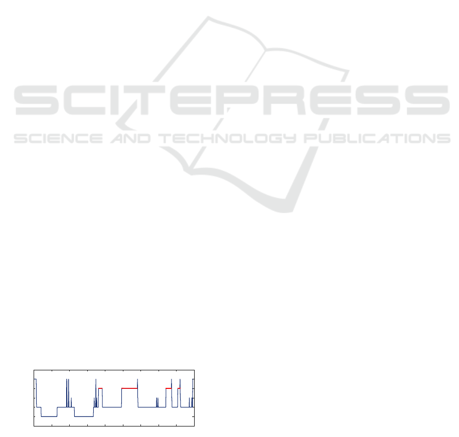
quence of stage labels is known as a hypnogram.
See Fig. 1 for a sample hypnogram from the sleep
database used in the present paper.
0 100 200 300 400 500 600 700 800 900
SWS
NREM 2
NREM 1
REM
wake
Time (epochs)
Sleep stage
Figure 1: Sample hypnogram from the present study.
The dynamics of sleep stage transitions are af-
fected by overall health (Burns et al., 2008), (Bianchi
et al., 2010), making dynamics a clinically important
aspect of sleep structure. The study of sleep stage dy-
namics involves the construction of dynamical mod-
els of discrete time series. A challenge that arises
in this context is the scarcity of key events in the
data: each data instance (all-night hypnogram) con-
tains on the order of 10
3
individual sleep stage labels,
but only a small number of actual transitions between
stages. Because of this, the information in a full night
hypnogram may be insufficient to adequately model
the dynamics of sleep stage transitions (Bianchi et al.,
2010). The present paper proposes a new approach
for addressing this problem, based on simultaneous
clustering and dynamical modeling of data. The ap-
plications of the proposed technique extend beyond
the study of sleep, to other domains that present in-
frequently changing discrete time series.
1.1 Related Work
Clustering for time-series data has been a topic of
great interest (e.g., (Liao, 2005)). Previous works
have addressed clustering of Markov chains (Ramoni
et al., 2001), (Cadez et al., 2003), hidden Markov
models (HMM) (Smyth, 1997), impulse-response
curves (Sivriver et al., 2011), or more general dynam-
ical models (Cadez et al., 2000). Some of these prior
works rely on modeling individual instances, for ex-
ample by constructing individual Markov chain mod-
els (Ramoni et al., 2001), or optimizing the parame-
209
A. Alvarez S. and Ruiz C..
Collective Probabilistic Dynamical Modeling of Sleep Stage Transitions.
DOI: 10.5220/0004243102090214
In Proceedings of the International Conference on Bio-inspired Systems and Signal Processing (BIOSIGNALS-2013), pages 209-214
ISBN: 978-989-8565-36-5
Copyright
c
2013 SCITEPRESS (Science and Technology Publications, Lda.)

ters of an instance-specific fit function (Sivriver et al.,
2011). Such an approach is not well-suited for the
event-sparse data in sleep studies, as the temporal in-
formation available per instance is insufficient for re-
liable statistical modeling (Bianchi et al., 2010).
The simultaneous modeling and clustering strat-
egy of the present paper is similar to that of (Sivriver
et al., 2011) for gene expression. However, the clus-
tering step in (Sivriver et al., 2011) involves estima-
tion of instance-specific parameters, a process that is
subject to high variance in the presence of small data
instances as considered here. In other prior work,
the application domain provides abundant temporal
information for each instance, as in the web navi-
gation data of (Cadez et al., 2003). The more gen-
eral E-M framework on which (Cadez et al., 2003)
is based (Dempster et al., 1977) does allow for an ap-
proach that applies in the present context, as described
below in section 2. A related approach in which indi-
viduals are clustered, allowing multiple instances for
each individual, is pursued in (Cadez et al., 2000). A
relevant alternative view of model-based clustering in
terms of a bipartite graph that connects instances with
generative models as generalized cluster centroids,
using the generative data likelihood as a proximity
measure, is presented in (Zhong and Ghosh, 2003).
2 METHODS
2.1 Markov Mixture Data
Preliminary experiments were performedon data gen-
erated by a Markov chain mixture model. Two or
three Markov chains, M
1
,···M
k
(k = 2 or k = 3), were
used, each over a two-element state space that can be
loosely associated with wake and sleep states. The
initial state is assumed to be wake for all generated
sequences. For each integer i between 1 and a desired
total number of sequences, N, an equiprobable choice
was made among the Markov chains M
1
,···M
k
. The
selected model was then used to generate an observa-
tion sequence of the desired length, L, which was used
as the i-th output sequence of the mixture model. The
values N = 50 and L = 100 were used in most trials.
2.2 Human Sleep Data
875 anonymized human polysomnographic record-
ings were obtained with IRB approval from the Sleep
Clinic at Day Kimball Hospital in Putnam, Connecti-
cut, USA. The recordings were staged in 30-second
epochs by trained sleep technicians using the R & K
standard (Rechtschaffen and Kales, 1968). R & K
NREM stages 3 and 4 were then combined to obtain
a single slow wave sleep (SWS) stage. This proce-
dure yields stage labels that are known (Moser et al.,
2009) to closely approximate the more recently pro-
posed AASM staging standard (Iber et al., 2007).
2.2.1 Sleep Data Descriptions
Three different versions of the human sleep dataset
are considered in the present paper, each correspond-
ing to a different description of the hypnogram time-
series that comprise the dataset.
Uncompressed Dataset. The uncompressed data
description uses full-length sequences of the standard
stage labels wake, N1, N2, SWS, REM. The large di-
mensionality of the uncompressed description leads
to long running times for Algorithm 1, and makes
convergence more difficult. For this reason, exper-
iments involving the uncompressed data description
required reduction of the size of the dataset through
random sampling. 105 instances were used.
WNR and WLD Datasets. In the two compressed
sleep data descriptions, each stage bout is replaced by
a single occurrence of the stage in question. For ex-
ample, the subsequence wake, wake, wake, N1, N1,
N2, SWS, SWS becomes N1, N2, SWS. The bout
duration information is stored separately. Additional
compression is then performed by reducing the num-
ber of distinct stages considered from five to three.
• The Wake/NREM/REM (WNR) dataset combines
the three stages N1, N2, SWS into a single NREM
stage, yielding the stages Wake, NREM, REM.
• The Wake/Light/Deep (WLD) dataset combines
the three stages N1, N2, REM into a single Light
sleep stage, yielding stages Wake, Light, SWS.
Use of the WNR and WLD datasets leads to a substan-
tial reduction in computing time as compared with
the uncompressed dataset, and facilitates convergence
of the CDMC Algorithm, allowing experiments to be
performed over the full set of 875 hypnograms.
2.3 The Collective Dynamical
Modeling-Clustering (CDMC)
Algorithm
The core of the approach proposed in the present
paper is the simultaneous clustering and dynamical
modeling technique described in pseudocode in Algo-
rithm 1. In the case of sleep, the instances of the input
dataset D will be sequences of sleep stage labels from
the datasets described in section 2.2.1.
BIOSIGNALS2013-InternationalConferenceonBio-inspiredSystemsandSignalProcessing
210

2.3.1 Main Steps in Algorithm 1
The proposed technique simultaneously learns a set
of dynamical models (cluster prototypes) and a cor-
responding cluster labeling, by alternating between
model estimation and clustering steps, terminating
when the cluster labelings change very little.
• Model estimation (
learnMLProtoypes
) learns a
maximum data likelihood dynamicalmodel M
i
for
each cluster C
i
.
• Clustering (
learnMLClusterLabels
): assigns
each instance x to the cluster c(x) having the
model M
c(x)
most likely to generate x.
2.3.2 Dynamical Model Types in Algorithm 1
Algorithm 1 encompasses not only standard HMM,
but also other types of dynamical models M for which
procedures are available for calculation of the gen-
erative likelihood P(x|M) and for maximum likeli-
hood model estimation. In particular, semi-Markov
models are included, which we are pursuing in work
in progress in order to capture the non-exponentially
distributed bout durations observed in certain human
sleep stages (Bianchi et al., 2010), (Lo et al., 2002).
2.4 Evaluation
Algorithm 1 was evaluated using hidden Markov
models (HMM) as the dynamical models, with the
Baum-Welch algorithm (e.g., (Rabiner, 1989)) for
HMM training in the
learnMLPrototypes
function,
the Rand index (Rand, 1971) to measure clustering
similarity in the stopping criterion, and a pseudo-
random initial cluster labeling c
0
. Fully observable
Markov chains were used as the dynamical models
in additional experiments over the compressed sleep
data representations (section 2.2.1). Results appear
in section 3. All implementations were carried out in
MATLAB
R
(The MathWorks, 2012).
2.4.1 Cluster Separation
Separation between clusters was measured by the log
likelihood margin (LLM) – the difference in log likeli-
hood between the first and second highest likelihood
cluster labels for each instance. Higher mean LLM
values indicate better cluster separation.
2.4.2 Statistical Significance
Population means were compared using a paired t-
test when the requisite normality assumption holds.
In other cases, a Wilcoxon rank sum test was used to
compare medians.
3 RESULTS
3.1 Markov Mixture Data
3.1.1 Two Generative HMM
Mixture data was obtained by an equiprobable selec-
tion between two generative HMM, each with two
states. For such HMM, the transition matrices are
completely determined by their values along the main
diagonal. Multiples of the identity matrix were used
for simplicity. 50 sequences of length 100 were gener-
ated per trial. 100 independent trials were performed.
Time to Convergence. The observed distribution
of the number of iterations for convergence of Algo-
rithm 1 with two clusters is nearly unimodal, with me-
dian and mode of 3 iterations, mean value of 3.72, and
standard deviation of 1.47. Over 90% of trials con-
verge in 5 or fewer iterations. With three clusters, me-
dian convergence time increases to 4 iterations, and
the 90th percentile increases to 7 iterations.
Variation with Initial Conditions. 100 trials were
performed with pseudorandom initial cluster la-
bels. HMM transition matrices T with diagonals
(T(1, 1),T(2,2)) of (0.6,0.6) and (0.75,0.75) were
used in the mixture model that generates the training
data. Mean ± std observed cluster centroids resulting
after convergence of Algorithm 1 are (0.66,0.64) ±
(0.036, 0.033) and (0.76,0.76) ± (0.020,0.021), re-
spectively, which fit the generative model well.
Dependence on Separation between Generative
HMM. Fig. 2 shows clustering results obtained
when one of the two generative matrices has diago-
nal elements (0.6,0.6). The other matrix has diago-
nal elements (0.75, 0.75). Each instance is displayed
at the point (
˜
T(1,1),
˜
T(2,2)), where
˜
T is the transi-
tion matrix for that instance as learned by the Baum-
Welch algorithm. The single instance for which the
CDMC algorithm (Algorithm 1) produces a labeling
error appears darker in the figure. The number of la-
beling errors increases as the separation between the
two generative HMM decreases: no labeling errors
occur when the generative diagonal values are 0.6,
0.85 instead of 0.6, 0.75, while many errors occur
with diagonal values 0.6, 0.65, for example.
3.1.2 Three Generative HMM. Determination of
the Number of Clusters.
Experiments were performed over mixture data pro-
duced by an equiprobable selection among 3 dist-
CollectiveProbabilisticDynamicalModelingofSleepStageTransitions
211
Algorithm 1: Collective Dynamical Modeling-Clustering (CDMC).
Input: An unlabeled time-series dataset D = {x = (a
t
(x)) | t = 1,2,3,...n}; a positive integer,
k, for the desired number of clusters; an initial guess c
0
: D → {1,···k} of the cluster label
c
0
(x) of each instance x ∈ D; parameter values, s, specifying the desired configuration of the
models (e.g., number of states); and a real number
minSim
between 0 and 1 for the minimum
clustering similarity required for stopping.
Output: A set M
1
,···M
k
of generative dynamical models (with configuration parameters s),
together with a cluster labeling c : D → {1· · · k} that associates to each data instance, x, the
index c(x) of a model M = M
c(x)
for which the generative likelihood
∏
x∈D
P(x|M
c(x)
) is as
high as possible.
CDMC(D,k,c
0
,s,
minSim
)
(1) c(x) = c
0
(x) for all x in D
(2) c
old
(x) = 0 for all x ∈ D
(3) while CLUSTERINGSIMILARITY(c,c
old
) <
minSim
(4) c
old
= c
(5) (M
1
,···M
k
) = LEARNMLPROTOYPES(D,k, c,s)
(6) c = LEARNMLCLUSTERLABELS(D,M
1
···M
k
)
(7) return M
1
,···M
k
,c
Figure 2: CDMC results (0.6,0.75 self-transition probabili-
ties). Triangles indicate learned cluster models.
inct generative HMM. 50 sequences of length 100
were used in each of 50 independent trials. Using 2
clusters in the CDMC algorithm, the observed mean
LLM (2.4.1) is approximately 9.9, which corresponds
to a likelihood ratio of approximately 2 10
4
. With 3
clusters, mean LLM increases to 10.1, which is sig-
nificantly greater than for 2 clusters as assessed by a
paired t-test using 50 paired trials (p < 0.02). Use
of a paired t-test is justified here because the LLM
distribution is close to normal except at the far tails,
as observed in a quantile-quantile plot (not shown
due to space restrictions). Specifying 4 clusters leads
to a statistically significant decrease in mean LLM
(p < 0.001). See Table 1. Thus, the number of gen-
erative models can be determined by maximizing the
LLM in the clustering results. These facts show that
the CDMC algorithm is able to uncover the statistical
structure that underlies the data generation process.
Table 1: Log-likelihood margin. 3-HMM mixture data.
number of clusters 2 3 4
mean LLM 9.87 10.07 6.83
3.2 Human Sleep Data
We summarize here the results obtained using the
CDMC algorithm (Algorithm 1) on the human sleep
data described in section 2.2.
3.2.1 HMM over Uncompressed Sleep Sample
We applied Algorithm 1 to a sample of 105 instances
drawn randomly from the human sleep dataset de-
scribed in section 2.2, with k = 2 clusters and a pseu-
dorandom initial choice of cluster labels. The algo-
rithm converges in a dozen or so iterations of the main
loop on average. The models learned in one of these
runs are visualized in Fig. 3. HMM with 2 states were
used, with 5 possible emitted symbols corresponding
to sleep stages 1, 2, SWS, REM, and wakefulness.
The left subplot displays individual data instances as
the diagonal elements of the 2× 2 state transition ma-
trices learned from them by Baum-Welch, with mark-
ers indicating cluster membership. The middle and
right subplots display the emission probability matri-
ces for the HMM models of the two clusters; the two
rows of each emission matrix are represented by the
solid and dashed lines in the lower subplots.
Observations. As observed in the left subplot in
Fig. 3, the diagonal elements of the individual state
BIOSIGNALS2013-InternationalConferenceonBio-inspiredSystemsandSignalProcessing
212
0.9 0.95 1
0.85
0.9
0.95
1
trans(1,1)
trans(2,2)
1 2 SWS REM wake
0
0.5
1
cluster1
log P(stage | state)
1 2 SWS REM wake
0
0.5
1
cluster2
1
2
Figure 3: HMM transition matrices (left) and emission probabilities (right), Markov mixture data.
Table 2: Iterations to convergence. 10 trials, two clusters.
WNR 2 5 14 4 10 3 2 3 9 16
WLD 2 4 2 2 2 2 5 21 5 4
Table 3: HSMM transition matrices, two clusters (WNR).
0.0000 0.9565 0.0435 0.0000 1.0000 0.0000
0.7879 0.0000 0.2121 0.9979 0.0000 0.0021
0.7864 0.2136 0.0000 1.0000 0.0000 0.0000
transition matrices are very close to 1, making it dif-
ficult to distinguish between clusters based on tran-
sition probabilities alone (diagonal mean and me-
dian differences are not statistically significant by a
Wilcoxon rank sum test). This is due to the long
average duration of stage bouts in comparison with
the HMM clock period. In the remainder of the
present paper, we address this modeling disadvantage
of Markov dynamics by using compressed datasets
(section 2.2.1), in which repetitions are eliminated
from the stage sequences. In work in progress, this is-
sue is resolved as a by-product of using semi-Markov
models, which represent the durations of state vis-
its explicitly by their distributions, rather than by a
period-by-period coin flip as Markov models do.
Comparing the subplots on the right in Fig. 3, we
see that the collective HMM for cluster 2 is more
likely to emit stage SWS than is the cluster 1 model.
The observed differences in stage SWS probabilities
are statistically significant (p < 0.05, using a bino-
mial model). Thus, the emission probabilities provide
separation between the clusters. Within each cluster
model, the states have specialized to correspond to
particular combinations of sleep stages. For exam-
ple, only the states with solid lines in these plots have
nonzero wake emission probability (p < 0.05).
3.2.2 Observable Markov Chains over
Compressed Sleep Data Representations
Wake–NREM–REM Data Representation. In
contrast with Markov mixture data (section 3.1), for
WNR sleep data the observed LLM (section 2.4)
distribution deviates substantially from normality.
Table 4: HSMM transition matrices, two clusters (WLD).
0 1.0000 0.0000 0.0000 0.9997 0.0003
0.9734 0 0.0266 0.6919 0.0000 0.3081
0.5389 0.4611 0 0.4668 0.5332 0.0000
The median LLM for the WNR data is roughly 6.4,
which corresponds to a likelihood ratio of 600: the
maximum likelihood cluster is 600 times as probable
as the next best cluster. For a WNR sequence
of median length 34, this equates to 20% higher
generative probability per symbol (e
6.4/34
≈ 1.2).
Sample learned WNR transition matrices (Table 3)
show dynamical differences between clusters: higher
NREM to REM and REM to NREM probabilities in
cluster 1 (left matrix, middle and bottom rows).
Wake–Light–Deep Data Representation. Table 2
compares the WNR and WLD convergence times in
ten trials, with a minimum Rand index of 0.95 as the
stopping criterion. The median and mean of 3 and 4.9
iterations for WLD data are slightly lower than the
corresponding WNR values, 4.5 and 6.8.
Typical transition matrices obtained by Algo-
rithm 1 over WLD data appear in Table 4. A wake
state is followed by light sleep with near certainty
(top row). However, while the first cluster exhibits
a very high probability of a light sleep to wake tran-
sition (left matrix, middle row), the second cluster
shows a substantial probability of transitioning from
light sleep to deep sleep (right matrix, middle row).
The distribution of the state immediately after a deep
sleep state (bottom row) is similar for the two clusters.
The LLM distribution for the WLD data is qualita-
tively similar to that for the WNR data. However, the
observed median LLM is approximately 3.5, corre-
sponding to a likelihood ratio of approximately 33, or
roughly 10% greater generative probability per sym-
bol for a typical WLD sequence of median length
37 (e
3.5/37
≈ 1.1). Thus, the WLD cluster separa-
tion is less pronounced than for the WNR data (c.f.
section 3.2.2). This suggests preferential use of the
WNR sleep data description in future work.
CollectiveProbabilisticDynamicalModelingofSleepStageTransitions
213

4 CONCLUSIONS; FUTURE
WORK
This paper has proposed a technique for dynamical
modeling of time-series with infrequent changes, and
has applied it to the study of human sleep data. The
technique, collective dynamical modeling and clus-
tering (CDMC), is based on adaptive pooling of data,
through iteration of clustering and dynamical mod-
eling steps. CDMC is a general algorithm that al-
lows a variety of probabilistic state space paradigms
(e.g., Markov chains, HMM, semi-Markov chains,
and HSMM) to be used as the dynamical models. Re-
sults over Markov mixture data show that the CDMC
algorithm converges rapidly, and that it successfully
identifies the statistical structure underlying the data
generation process. Preliminary results have been ob-
tained over human sleep data, using a compressed
data representation that captures the temporal order-
ing of stage transitions but not the stage bout dura-
tions. These results demonstrate convergence of the
CDMC algorithm over real clinical data, with good
cluster separation. The clusters found are shown to be
characterized by distinct sleep-dynamical properties.
Work in progress by the authors builds on the
present paper by including detailed stage bout timing
information, using semi-Markov chains as the spe-
cific dynamical models in the CDMC algorithm. In
future work, there will be a need to systematically as-
sess convergence, as well as clustering stability with
respect to initial parameter values. The effect on
convergence of alternative strategies for initialization
should also be examined. The applications to sleep
dynamics of the CDMC algorithm proposed in the
present paper should be explored in greater detail.
REFERENCES
Bianchi, M. T., Cash, S. S., Mietus, J., Peng, C.-K.,
and Thomas, R. (2010). Obstructive sleep apnea al-
ters sleep stage transition dynamics. PLoS ONE,
5(6):e11356.
Burns, J. W., Crofford, L. J., and Chervin, R. D. (2008).
Sleep stage dynamics in fibromyalgia patients and
controls. Sleep Medicine, 9(6):689–696.
Cadez, I., Gaffney, S., and Smyth, P. (2000). A general
probabilistic framework for clustering individuals. In
In Proceedings of the sixth ACM SIGKDD Interna-
tional Conference on Knowledge Discovery and Data
Mining, pages 140–149.
Cadez, I., Heckerman, D., Meek, C., Smyth, P., and White,
S. (2003). Model-based clustering and visualization of
navigation patterns on a web site. Data Min. Knowl.
Discov., 7:399–424.
Cavallero, C., Cicogna, P., Natale, V., Occhionero, M., and
Zito, A. (1992). Slow wave sleep dreaming. Sleep,
15(6):562–6.
Dempster, A. P., Laird, N. M., and Rubin, D. B. (1977).
Maximum likelihood from incomplete data via the
EM algorithm. Journal of the Royal Statistical So-
ciety, Series B, 39(1):1–38.
Iber, C., Ancoli-Israel, S., Chesson, A., and Quan, S.
(2007). The AASM Manual for the Scoring of Sleep
and Associated Events: Rules, Terminology, and Tech-
nical Specifications. American Academy of Sleep
Medicine, Westchester, Illinois, USA.
Liao, T. W. (2005). Clustering of time series data – a survey.
Pattern Recognition, 38(11):1857 – 1874.
Lo, C.-C., Amaral, L. A. N., Havlin, S., Ivanov, P. C., Pen-
zel, T., Peter, J.-H., and Stanley, H. E. (2002). Dynam-
ics of sleep-wake transitions during sleep. Europhys.
Lett., 57(5):625–631.
Moser, D., Anderer, P., Gruber, G., Parapatics, S., Loretz,
E., Boeck, M., Kloesch, G., Heller, E., Schmidt,
A., Danker-Hopfe, H., Saletu, B., Zeitlhofer, J., and
Dorffner, G. (2009). Sleep classification according to
AASM and Rechtschaffen & Kales: Effects on sleep
scoring parameters. Sleep, 32(2):139–149.
Rabiner, L. R. (1989). A tutorial on hidden markov models
and selected applications in speech recognition. Pro-
ceedings of the IEEE, 77(2):257–286.
Ramoni, M., Sebastiani, P., and Cohen, P. (2001). Bayesian
clustering by dynamics. Machine Learning, pages 1–
31.
Rand, W. M. (1971). Objective criteria for the evaluation of
clustering methods. Journal of the American Statisti-
cal Association, 66(336):846–850.
Rechtschaffen, A. and Kales, A., editors (1968). A Manual
of Standardized Terminology, Techniques, and Scor-
ing System for Sleep Stages of Human Subjects. US
Department of Health, Education, and Welfare Public
Health Service – NIH/NIND.
Sivriver, J., Habib, N., and Friedman, N. (2011). An
integrative clustering and modeling algorithm for
dynamical gene expression data. Bioinformatics,
27(13):i392–i400.
Smyth, P. (1997). Clustering sequences with hidden
Markov models. In Mozer, M. C., Jordan, M. I., and
Petsche, T., editors, Advances in Neural Information
Processing 9, pages 648–654. MIT Press.
Zhong, S. and Ghosh, J. (2003). A unified framework
for model-based clustering. J. Mach. Learn. Res.,
4:1001–1037.
BIOSIGNALS2013-InternationalConferenceonBio-inspiredSystemsandSignalProcessing
214
