
Forecasting for Discrete Time Processes based on Causal Band-limited
Approximation
Nikolai Dokuchaev
Department of Mathematics & Statistics, Curtin University, GPO Box U1987, Perth, 6845 Western Australia, Australia
Keywords:
Band-limited Processes, Discrete Time Processes, Causal Filters, Low-pass Filters, Forecasting.
Abstract:
We study causal dynamic smoothing of discrete time processes via approximation by band-limited discrete
time processes. More precisely, a part of the historical path of the underlying process is approximated in Eu-
clidean norm by the trace of a band-limited process. We analyze related optimization problem and obtain some
conditions of solvability and uniqueness. An unique extrapolation to future times of the optimal approximating
band-limited process can be interpreted as an optimal forecast.
1 INTRODUCTION
We study causal dynamic smoothing of discrete time
processes via approximation by band-limited discrete
time processes. More precisely, a part of the historical
path of the underlying process is approximated in Eu-
clidean norm by the trace of a band-limited discrete
time process. Since an unique extrapolation to fu-
ture times of the optimal approximating band-limited
process can be interpreted as an optimal forecast, this
task has many practical applications. It is well known
that it is not possible to find an ideal low-pass causal
linear time-invariant filter. In continuous time setting,
it is known that the distance of the set of ideal low-
pass filters from the set of all causal filters is positive
(Almira and Romero, 2008) and that the optimal ap-
proximation of the ideal low-pass filter is not possible
(Dokuchaev, 2012c). Our goal is to substitute the so-
lution of these unsolvable problems by solution of an
easier problem in discrete time setting such that the
filter is not necessary time invariant. Our motivation
is that, for some problems, the absence of time in-
variancy for a filter can be tolerated. For example,
a typical approach to forecasting in finance is to ap-
proximate the known path of the stock price process
by a process allowing an unique extrapolation that can
be used as a forecast. This has to be done at current
time; at future times, forecasting rule can be amended
according to new data collected.
We suggest to approximate discrete time pro-
cesses by the discrete time band-limited processes.
More precisely, we suggest to approximate the known
historical path of the process by the trace of a band-
limited process. The approximating sequence does
not necessary match the underlying process at sam-
pling points. This is different from classical sampling
approach; see, e.g., (Jerry, 1977). Our approach is
close to the approach from (Ferreira, 1995b) and (Fer-
reira, 1995a), where the estimate of the error norm is
given. The difference is that, in our setting, it is guar-
anteed that the approximation generates the error of
the minimal Euclidean norm.
We obtain analyze existence and uniqueness of an
optimal approximation. The optimal process is de-
rived in time domain in a form of sinc series.The ap-
proximating band-limited process can be interpreted
as a causal and linear filter that is not time invari-
ant. The filter obtained is not time invariant; as a
consequence, the coefficients of these series and have
to be changed dynamically, to accommodate the cur-
rent flow of observations. An unique extrapolation
to future times of the optimal approximating band-
limited process can be interpreted as an optimal fore-
cast at any given time. This paper develops further the
approach suggested in (Dokuchaev, 2011) where the
continuous time setting was considered. We extend
now this approach on discrete time processes. Some
related results can be found in (Dokuchaev, 2012b)
and (Dokuchaev, 2012d) for discrete time processes
that are band-limited or close to band-limited.
2 DEFINITIONS
For a Hilbert space H, we denote by (·,·)
H
the cor-
280
Dokuchaev N..
Forecasting for Discrete Time Processes based on Causal Band-limited Approximation.
DOI: 10.5220/0004243700820085
In Proceedings of the 2nd International Conference on Operations Research and Enterprise Systems (ICORES-2013), pages 82-85
ISBN: 978-989-8565-40-2
Copyright
c
2013 SCITEPRESS (Science and Technology Publications, Lda.)

responding inner product. We use notation sinc(x) =
sin(x)/x.
Let Z be the set of all integers, and let Z
+
be the
set of all positive integers. We denote by ℓ
r
the set
of all sequences x = {x(t)}
t∈Z
⊂ R, such that kxk
ℓ
r
=
∑
∞
t=−∞
|x(t)|
r
1/r
< +∞ for r ∈ [1, ∞) or for r = +∞.
Let ℓ
+
r
be the set of all sequences x ∈ ℓ
r
such that
x(t) = 0 for t = −1,−2,−3,....
For x ∈ ℓ
1
or x ∈ ℓ
2
, we denote by X = Z x the
Z-transform
X(z) =
∞
∑
t=−∞
x(t)z
−t
, z ∈ C.
Respectively, the inverse Z-transform x = Z
−1
X is de-
fined as
x(t) =
1
2π
Z
π
−π
X
e
iω
e
iωt
dω, t = 0,±1,±2,....
If x ∈ ℓ
2
, then X|
T
is defined as an element of
L
2
(T).
Let θ,τ ∈ Z ∪ {+∞} and θ < τ. We de-
note by ℓ
2
(θ,τ) the Hilbert space of complex
valued sequences {x(t)}
τ
t=θ
such that kxk
ℓ
2
(θ,τ)
=
∑
τ
t=θ
|x(t)|
2
1/2
< +∞.
Let U
Ω,∞
be the set of all mappings X : T → C
such that X
e
iω
∈ L
2
(−π,π) and X
e
iω
= 0 for
|ω| > Ω. Note that the corresponding processes x =
Z
−1
X are said to be band-limited.
Let U
Ω,N
be the set of all X ∈ U
Ω,∞
such that
there exists a sequence {y
k
}
N
k=−N
∈ C
2N+1
such that
X
e
iω
=
∑
N
k=−N
y
k
e
ikω/Ω
I
{|ω|≤Ω}
, where I is the in-
dicator function.
We assume that we are given Ω ∈ (π/2,π), N ∈
Z
+
, s ∈ Z and q ∈ Z, such that q < s and s − q ≥
2N + 1.
Let T = {t ∈ Z : q ≤ t ≤ s}.
Let Z
N
be the set of all integers k such that |k| ≤ N.
Let Y
N
be the Hilbert space of sequences
{y
k
}
N
k=−N
⊂ C provided with the Euclidean norm, i.e.,
such that kyk
Y
N
=
∑
k∈Z
N
|y
k
|
2
1/2
.
Consider the Hilbert spaces of sequences X = ℓ
2
and X
−
= ℓ
2
(q,s).
Let X
Ω,N
be the subset of X
−
consisting of se-
quences {x(t)}|
t∈T
, where x ∈ X are such that x(t) =
(Z
−1
X)(t) for t ∈ T for some X
e
iω
∈ U
Ω,N
.
Up to the end of this paper, we assume that the
following condition is satisfied.
Condition 2.1. The matrix {sinc(kπ + Ωm)}
N
k,m=−N
is nondegenerate.
Lemma 1. Let Ω
0
∈ (π/2,π) be selected such that
there exists p ∈ (0,1) such that
min
k∈Z
N
|sinc(πk− Ωk)| ≥ p,
max
k,m∈Z
N
, t6=−k
|sinc(πk+ Ωm)| <
p
2N
for all Ω ∈ [Ω
0
,π). (1)
Then the matrix {sinc(kπ + Ωm)}
N
k,m=−N
is nonde-
generate for all Ω ∈ [Ω
0
,π).
Clearly, (1) holds for any Ω
0
that is close enough
to π, since sinc(x) → 1 as x → 0 and sinc(x) → 0 as
x → πm, where m ∈ Z, m 6= 0. Therefore, Condition
2.1 can be satisfied with selection of Ω being close
enough to π.
Lemma 2. For any any x ∈ X
Ω,N
, there exists an
unique X ∈ U
Ω,N
such that x(t) = (Z
−1
X)(t).
By Lemma 2, the future of even more ”smooth”
processes from X
Ω,N
is uniquely defined by a finite set
of historical values that has at least 2N + 1 elements
for any N < +∞ and Ω ∈ [Ω
0
,π).
3 APPROXIMATION RESULTS
3.1 The Optimization Problem in the
Time Domain
Let x ∈ X be a process. We assume that the sequence
{x(t)}
t∈T
represents available historical data. Let
Hermitian form F : X
Ω,N
× X
−
→ R be defined as
F(bx,x) =
s
∑
t=q
|bx(t) − x(t)|
2
.
Theorem 1. (i) There exists an optimal solution bx of
the minimization problem
Minimize F(bx,x) over bx ∈ X
Ω,N
. (2)
(ii) If s− q ≥ 2N + 1, then the corresponding optimal
process bx is uniquely defined.
Remark 1. By Proposition 2, there exists an unique
extrapolation of the band-limited solution bx of prob-
lem (2) on the future times t > s, under the assump-
tions of Theorem 1. It can be interpreted as the opti-
mal forecast (optimal given Ω and N).
3.2 The Optimization Problem for
Fourier Coefficients
To solve problem (2) numerically, it is convenient
to expand Z-transform X
e
iω
on the unit circle via
Fourier series.
ForecastingforDiscreteTimeProcessesbasedonCausalBand-limitedApproximation
281

Consider the mapping Q : Y
N
→ X
Ω,N
such that
bx = Q y is such that bx(t) = (Z
−1
b
X)(t) for t ∈ (q,s],
where
b
X
e
iω
=
∑
k∈Z
N
y
k
e
ikω/Ω
I
{|ω|≤Ω}
. (3)
Clearly, this mapping is linear and continuous.
Let Hermitian form G : Y
N
× X
−
→ R be defined
as
G(y,x) = F(Q y, x) =
s
∑
t=q
|bx(t) − x(t)|
2
,
bx = Q y. (4)
Corollary 1. There exists an unique solution y of the
minimization problem
Minimize G(y,x) over y ∈ Y
N
. (5)
Problem (2) can be solved via problem (5); its so-
lution can be found numerically.
Let
b
X be defined by (3), where {y
k
} ∈ Y
N
. Let
bx = Z
−1
b
X. We have that
bx(t) =
1
2π
Z
Ω
−Ω
∑
k∈Z
N
y
k
e
ikωπ/Ω
!
e
iωt
dω
=
1
2π
∑
k∈Z
N
y
k
Z
Ω
−Ω
e
ikωπ/Ω+iωt
dω
=
1
2π
∑
k∈Z
N
y
k
e
ikπ+iΩt
− e
−ikπ−iΩt
ikπ/Ω + it
=
Ω
π
∑
k∈Z
N
y
k
sinc(kπ + Ωt).
Hence
G(y,x) =
s
∑
t=q
|bx(t) − x(t)|
2
=
s
∑
t=q
Ω
π
∑
k∈Z
N
y
k
sinc(kπ + Ωt) − x(t)
2
= (y,Ry)
Y
N
− 2Re(y,rx)
X
−
+ (ρx,x)
X
−
. (6)
Here R : Y
N
× Y
N
→ Y
N
is a linear bounded Hermi-
tian operator, r : X
−
→ Y
N
is a bounded linear opera-
tor, ρ : X
−
× X
−
→ X
−
is a linear bounded Hermitian
operator.
It follows from the definitions that the operator
R is non-negatively defined (it suffices to substitute
x(t) ≡ 0 into the Hermitian form).
3.3 The Explicit Solution of the
Optimization Problem
Since the space Y
N
is finite dimensional, the opera-
tor R can be represented via a matrix R = {R
km
} ∈
C
2N+1,2N+1
, where R
km
= R
mk
. In this setting,
(Ry)
k
=
∑
N
k=−N
R
km
y
m
.
Theorem 2. (i) The operator R is positively defined.
(ii) Problem (5) has a unique solution by = R
−1
rx.
(iii) The components of the matrix R can be found from
the equality
R
km
=
Ω
2
π
2
s
∑
t=q
sinc(mπ + Ωt)sinc(kπ + Ωt). (7)
(iv) The components of the vector rx = {(rx)
k
}
N
k=−N
can be found from the equality
(rx)
k
=
Ω
π
s
∑
t=q
sinc(kπ + Ωt)x(t). (8)
Corollary 2. Let by be the vector calculated as in The-
orem 2, by = {by
k
}
N
k=−N
. The process
bx(t) = bx(t,q,s) =
Ω
π
∑
k∈Z
N
y
k
sinc(kπ + Ωt)
represents the output of a causal filter that is linear
but not time invariant.
The proofs of results given above can be found in
the working paper (Dokuchaev, 2012a).
4 NUMERICAL EXPERIMENTS
In the numerical experiments described below, we
have used MATLAB.
The experiments show that some eigenvalues of R
are quite close to zero despite the fact that, by The-
orem 2, R > 0. Respectively, the error for the MAT-
LAB solution of the equation Rby = rx does not vanish.
Further, in our experiments, we found that the error E
can be decreased by the replacing R in the equation
bx = R
−1
rx by R
ε
= R + εI, where I is the unit matrix
and where ε > 0 is small. We have used ε = 0.001.
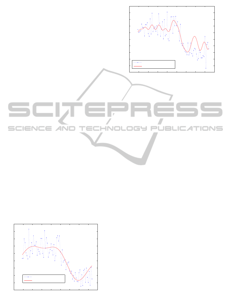
Figures 2 show examples of processes x(t) and
the corresponding band-limited processes bx(t) with
approximating x(t) with N = 15 at times t ∈
{−25, ...,15} (i.e., with q = −25, s = 15). The values
of bx(t) for t > 15 were calculated using { x(s)}
s≤15
and can be considered as an optimal forecast of x(t).
Figure 2 shows the result for Ω = 0.2; Figure ??
shows the result for Ω = 0.9.
We have verified numerically that the matrix
{sinc(kπ + Ωm)}
N
k,m=−N
is nondegenerate. There-
fore, Condition 2.1 is satisfied. In fact, we found that
this matrix was nondegenerate in all experiments for
all kinds of Ω and N.
By Remark 1, the extrapolation of the process bx ∈
X
Ω,N
to the future times t > s can be interpreted as the
optimal forecast (optimal given Ω and N).
ICORES2013-InternationalConferenceonOperationsResearchandEnterpriseSystems
282
ACKNOWLEDGEMENTS
This work was supported by ARC grant of Australia
DP120100928 to the author.
REFERENCES
Almira, J. and Romero, A. (2008). How distant is the ideal
filter of being a causal one? In Atlantic Electronic
Journal of Mathematics. 3 (1) 46–55.
Dokuchaev, N. (2011). On causal band-limited
mean square approximation. In Working paper.
http://arxiv.org/abs/1111.6701.
Dokuchaev, N. (2012a). Causal band-limited approxima-
tion and forecasting for discrete time processes. In
Working paper. http://lanl.arxiv.org/abs/1208.3278.
Dokuchaev, N. (2012b). On predictors for band-limited and
high-frequency time series. In Signal Processing. 92,
iss. 10, 2571-2575.
Dokuchaev, N. (2012c). On sub-ideal causal smoothing fil-
ters. In Signal Processing. 92, iss. 1, 219-223.
Dokuchaev, N. (2012d). Predictors for discrete time pro-
cesses with energy decay on higher frequencies. In
IEEE Transactions on Signal Processing. 60, No. 11,
6027-6030.
Ferreira, P. G. S. G. (1995a). Approximating non-band-
limited functions by nonuniform sampling series. In
SampTA’95.
Ferreira, P. G. S. G. (1995b). Nonuniform sampling of non-
bandlimited signals. In IEEE Signal Processing Let-
ters. 2, Iss. 5, 89–91.
Jerry, A. (1977). The shannon sampling theorem - its vari-
ous extensions and applications: A tutorial review. In
Proc. IEEE. 65, 11, 1565–1596.
APPENDIX
−40 −30 −20 −10 0 10 20 30 40 50
−0.6
−0.4
−0.2
0
0.2
0.4
0.6
0.8
1
1.2
t
original process
band−limited approximation
Figure 1: Example of x(t) and band-limited process bx(t)
approximating x(t) for t ∈ {−25,.., 15}, with Ω = 0.2, and
N = 15.
−40 −30 −20 −10 0 10 20 30 40 50
−0.8
−0.6
−0.4
−0.2
0
0.2
0.4
0.6
0.8
1
1.2
t
original process
band−limited approximation
Figure 2: Example of x(t) and band-limited process bx(t)
approximating x(t) for t ∈ {−25,..,15}, with Ω = 0.9, and
N = 15.
ForecastingforDiscreteTimeProcessesbasedonCausalBand-limitedApproximation
283
