
Applications of Discriminative Dimensionality Reduction
Barbara Hammer, Andrej Gisbrecht and Alexander Schulz
CITEC Centre of Excellence, Bielefeld University, Bielefeld, Germany
Keywords:
Dimensionality Reduction, Fisher Information Metric, Classifier Visualization, Evaluation.
Abstract:
Discriminative nonlinear dimensionality reduction aims at a visualization of a given set of data such that the
information contained in the data points which is of particular relevance for a given class labeling is displayed.
We link this task to an integration of the Fisher information, and we discuss its difference from supervised
classification. We present two potential application areas: speed-up of unsupervised nonlinear visualization
by integration of prior knowledge, and visualization of a given classifier such as an SVM in low dimensions.
1 INTRODUCTION
Caused by a rapid digitalization of almost all areas of
daily life, data sets and learning scenarios are increas-
ing dramatically with respect to both, size and com-
plexity. This fact poses new challenges for standard
data analysis tools: on the one hand, methods have
to deal with very large data sets such that many algo-
rithms rely on sampling or approximation techniques
to maintain feasibility (Bekkerman et al., 2011; Tsang
et al., 2005). Hence valid results have to be guaran-
teed based on a small subset of the full data only. On
the other hand, an exact objective is often not clear a
priori; rather, the user specifies her interests and de-
mands interactively when applying data mining tech-
niques and inspecting the results (Ward et al., 2010).
This places the human into the loop, causing the need
for intuitive interfaces to the machine learning scenar-
ios (Vellido et al., 2012; R
¨
uping, 2006). In turn, this
demand causes an additional need for fast and online
machine learning technology since the user is usually
not willing to wait for more than a few seconds until
she gets (at least preliminary) results.
The visual system constitutes one of our most ad-
vanced senses, and humans display astonishing cog-
nitive capabilities as concerns vision such as group-
ing of objects or instantaneous recognition of artifacts
in visual scenes. In consequence, visualization plays
an essential part in the context of interactive machine
learning. This causes the need for reliable, fast and
online visualization techniques of data and machine
learning results when training on the given data.
Dimensionality reduction refers to the specific
task to map high dimensional data points into low di-
mensions such that data can directly be displayed on
the screen while as much information as possible is
preserved. Classical techniques such as a simple prin-
ciple component analysis (PCA) offer a linear projec-
tion only, thus their flexibility is limited. Neverthe-
less, they are widely used today due to their excellent
generalization ability and scalability.
In recent years, a large variety of nonlinear alter-
natives has been proposed, formalizing the ill-posed
objective of what means ‘structure preservation’ via
different mathematical objectives. Popular examples
include techniques such as maximum variance un-
folding, non-parametric embedding, Isomap, locally
linear embedding (LLE), stochastic neighbor embed-
ding (SNE), and similar, see e.g. the overviews (Bunte
et al., 2012a; Lee and Verleysen, 2007; Maaten and
Hinton, 2008). These techniques, however, have sev-
eral drawbacks such that many practitioners still rely
on simpler linear techniques such as PCA (Biehl et al.,
2011): many nonlinear techniques provide a mapping
of the given data points only, requiring additional ef-
fort for out-of-sample extensions. Due to the inherent
ill-posedness of dimensionality reduction, the results
are not easily interpretable by humans and first for-
mal evaluation measures for dimensionality reduction
have just recently been proposed (Lee and Verleysen,
2010). Further, most techniques depend on pairwise
distances of data such that they scale at least quadrat-
ically with the data set size, making the techniques
infeasible for large data sets.
In this contribution, we consider a specific variant
of dimensionality reduction: discriminative dimen-
sionality reduction, i.e. the case where data are ac-
companied by additional labeling. In this setting, the
33
Hammer B., Gisbrecht A. and Schulz A. (2013).
Applications of Discriminative Dimensionality Reduction.
In Proceedings of the 2nd International Conference on Pattern Recognition Applications and Methods, pages 33-41
DOI: 10.5220/0004245300330041
Copyright
c
SciTePress

goal is to visualize those aspects of the data which
are of particular relevance for the given labeling. A
few approaches have been proposed in this context:
classical Fisher’s linear discriminant analysis (LDA)
projects data such that within class distances are min-
imized while between class distances are maximized,
still relying on a linear mapping. The objective of par-
tial least squares regression (PLS) is to maximize the
covariance of the projected data and the given auxil-
iary information. It is also suited if data dimension-
ality is larger than the number of data points. In-
formed projections (Cohn, 2003) extend PCA to min-
imize the sum squared error and the mean value of
given classes, this way achieving a compromise of di-
mensionality reduction and clustering. In (Goldberger
et al., 2004), the metric is adapted according to auxil-
iary class information prior to projection to yield a
global linear matrix transform. Further, interesting
extensions of multidimensional scaling to incorporate
class information have recently been proposed (Wit-
ten and Tibshirani, 2011). Modern techniques extend
these settings to general nonlinear projections of data.
One way is offered by kernelization such as kernel
LDA (Ma et al., 2007; Baudat and Anouar, 2000;
Mika et al., 1999). Another principled way to extend
dimensionality reducing data visualization to auxil-
iary information is offered by an adaptation of the un-
derlying metric. The principle of learning metrics has
been introduced in (Kaski et al., 2001; Peltonen et al.,
2004): the standard Riemanian metric is substituted
by a form which measures the information of the data
for the given classification task (Kaski et al., 2001;
Peltonen et al., 2004; Venna et al., 2010). A slightly
different approach is taken in (Geng et al., 2005), re-
lying on an ad hoc adaptation of the metric. Met-
ric adaptation based on the classification margin and
subsequent visualization has been proposed in (Bunte
et al., 2012b), for example. Alternative approaches
to incorporate auxiliary information modify the cost
function of dimensionality reducing data visualiza-
tion. The approaches introduced in (Iwata et al., 2007;
Memisevic and Hinton, 2005) can both be understood
as extensions of SNE. Multiple relational embedding
(MRE) incorporates several dissimilarity structures in
the data space induced by labeling, for example, into
one latent space representation. Colored MVU incor-
porates auxiliary information into MVU by substitut-
ing the raw data by the combination of the data and
the covariance matrix induced by the given auxiliary
information.
What are the differences of a supervised visual-
ization as compared to a direct classification of the
data, i.e. a simple projection of the data points to their
corresponding class labels? What are potential appli-
cations of such techniques? These questions are in
the focus of this contribution. We will argue that aux-
iliary information in the form of class labeling can
play a crucial role when addressing dimensionality re-
duction: on the one hand, it offers a natural way to
shape the inherently ill-posed problem of dimension-
ality reduction by explicitly specifying which aspects
of the data are relevant and, in consequence, which
aspects should be emphasized – those aspects of the
data which are relevant for the given auxiliary class
labeling. In addition, the integration of auxiliary in-
formation can help to solve the problem of the com-
putational complexity of dimensionality reduction. In
this contribution, we will show that discriminative di-
mensionality reduction can be used to infer a mapping
of points based on a small subsample of data only,
thus reducing the complexity by an order of magni-
tude. We will use this technique in a general frame-
work which allows us to visualize not only a given
labeled data set, rather full classification models can
be displayed this way, as we will demonstrate for the
case of SVM classifiers.
Now we will first introduce the Fisher metric as
a general way to include auxiliary class labels into
a non-linear dimensionality reduction technique. We
show the difference of the result from a direct clas-
sification in the context of discriminative t-SNE. Af-
terwards, we address two applications of this setting:
integration of auxiliary information into kernel t-SNE
mapping to obtain valid results from a small subset of
data only, and vizualisation of a given SVM classifier.
2 SUPERVISED VISUALIZATION
BASED ON THE FISHER
INFORMATION
In the following, we will consider only one proto-
typical dimensionality reduction technique and em-
phasize the role of discriminative visualization rather
than a comparison of the underlying dimensional-
ity reduction technique: we restrict to t-distributed
stochastic neighbor embedding (t-SNE), which con-
stitutes one of the most successful nonlinear dimen-
sionality reduction techniques used today (Maaten
and Hinton, 2008). All arguments as given below
could also be based on alternatives such as LLE or
Isomap.
Given a set of data points x
i
in some high-
dimensional data space X, t-SNE finds projections y
i
for these points in the two dimensional plane Y = R
2
such that the probabilities of data pairs in the original
space and the projection space are preserved as much
ICPRAM2013-InternationalConferenceonPatternRecognitionApplicationsandMethods
34

as possible. More precisely, probabilities in the orig-
inal space are defined as p
i j
= (p
(i| j)
+ p
( j|i)
)/(2N)
where N is the number of data points and
p
j|i
=
exp(−kx
i
− x
j
k
2
/2σ
2
i
)
∑
k6=i
exp(−kx
i
− x
k
k
2
/2σ
2
i
)
.
depends on the pairwise distance; σ
i
is automatically
determined by the method such that the effective num-
ber of neighbors coincides with a priorly specified
parameter, the perplexity. In the projection space,
probabilities are induced by the student-t distribution
rather than Gaussians
q
i j
=
(1 + ky
i
− y
j
k
2
)
−1
∑
k6=l
(1 + ky
k
− y
l
k
2
)
−1
.
to avoid the crowding problem by means of using a
long tail distribution. The goal is to find projection
points y
i
such that the difference between p
i j
and q
i j
becomes small as measured by the Kullback-Leibler
divergence. Usually, a gradient based optimization
technique is used to minimize these costs.
As mentioned already above, the goal of dimen-
sionality reduction is inherently ill-posed: in general,
there does not exist a loss-free representation of data
in two-dimensions, such that information loss is in-
evitable. Thereby, it depends on the users need which
type of information is relevant for the application. A
chosen dimensionality reduction technique implicitly
specifies which type of information is preserved by
means of specifying an abstract mathematical objec-
tive which is optimized while mapping. Such an ab-
stract cost function, however, is hardly accessible by
a user, and it cannot easily be altered according to
the users needs. Due to this fact, it has been pro-
posed e.g. in (Kaski et al., 2001; Peltonen et al., 2004;
Venna et al., 2010) to enhance data by auxiliary infor-
mation specified by the user which should be taken
into account while projecting. Formally, we assume
that every data point x
i
is equipped with a class label
c
i
which are instances of a finite number of possible
classes c. Now projection points y
i
should be found
such that the aspects of x
i
which are relevant for c
i
are
displayed.
How can this be realized? A Riemannian mani-
fold can easily be defined which is based on the in-
formation of x
i
for the class labels as metric tensor.
The tangent space at x
i
is equipped with the quadratic
form
d
x
i
(x,y) = x
T
J(x
i
)y
where J(x) denotes the Fisher information matrix
J(x) = E
p(c|x)
(
∂
∂x
log p(c|x)
∂
∂x
log p(c|x)
T
)
.
A Riemannian metric is induced by minimum path
integrals using this quadratic form locally, i.e.
d(x,y) = inf
p
Z
1
0
q
d
p(t)
(p
0
, p
0
)dt
where p : [0,1] → X ranges over all smooth curves
from p(0) = x to p(1) = y in X. We refer to this met-
ric as the Fisher metric in the following. Thus, auxil-
iary information can be integrated into t-SNE or any
other dimensionality reduction technique which relies
on distances by substituting the Euclidean metric by
the Fisher metric.
In how far is this technique different from a sim-
ple classification of data, i.e. in how far does a pro-
jection carry more information than a simple projec-
tion of the data to their distinct class labels? A very
simple example as shown in Fig. 1 illustrates the dif-
ference: Three classes which consist of two clusters
each are generated in two dimensions. Thereby, the
classes of two modes overlap (see arrow). We mea-
sure pairwise distances of these data using the Fisher
metric. These values are displayed using metric mul-
tidimensional scaling. As can be seen, the following
effects occur:
• the distance of data within a single mode belong-
ing to one class becomes smaller by scaling di-
mensions which are unimportant for a given la-
beling at a smaller scale. Thus, data points in one
clearly separated mode have the tendency to be
mapped on top of each other, and these cluster
structures become more apparent.
• the number of modes of the classes is preserved,
emphasizing the overall structure of the class dis-
tribution in space – unlike a simple mapping of
data to class labels which would map all modes of
one class on top of each other.
• overlapping classes are displayed as such (see ar-
row) and directions which cause this conflict are
preserved since they have an influence on the class
labeling. In contrast, a direct mapping of such
data to their class labels (if possible) would re-
solve such conflicts in the data.
In practice, the Fisher distance has to be estimated
based on the given data only. The conditional prob-
abilities p(c|x) can be estimated from the data using
the Parzen nonparametric estimator
ˆp(c|x) =
∑
i
δ
c=c
i
exp(−kx − x
i
k
2
/2σ
2
)
∑
j
exp(−kx − x
j
k
2
/2σ
2
)
.
The Fisher information matrix becomes
J(x) =
1
σ
4
E
ˆp(c|x)
b(x,c)b(x,c)
T
ApplicationsofDiscriminativeDimensionalityReduction
35
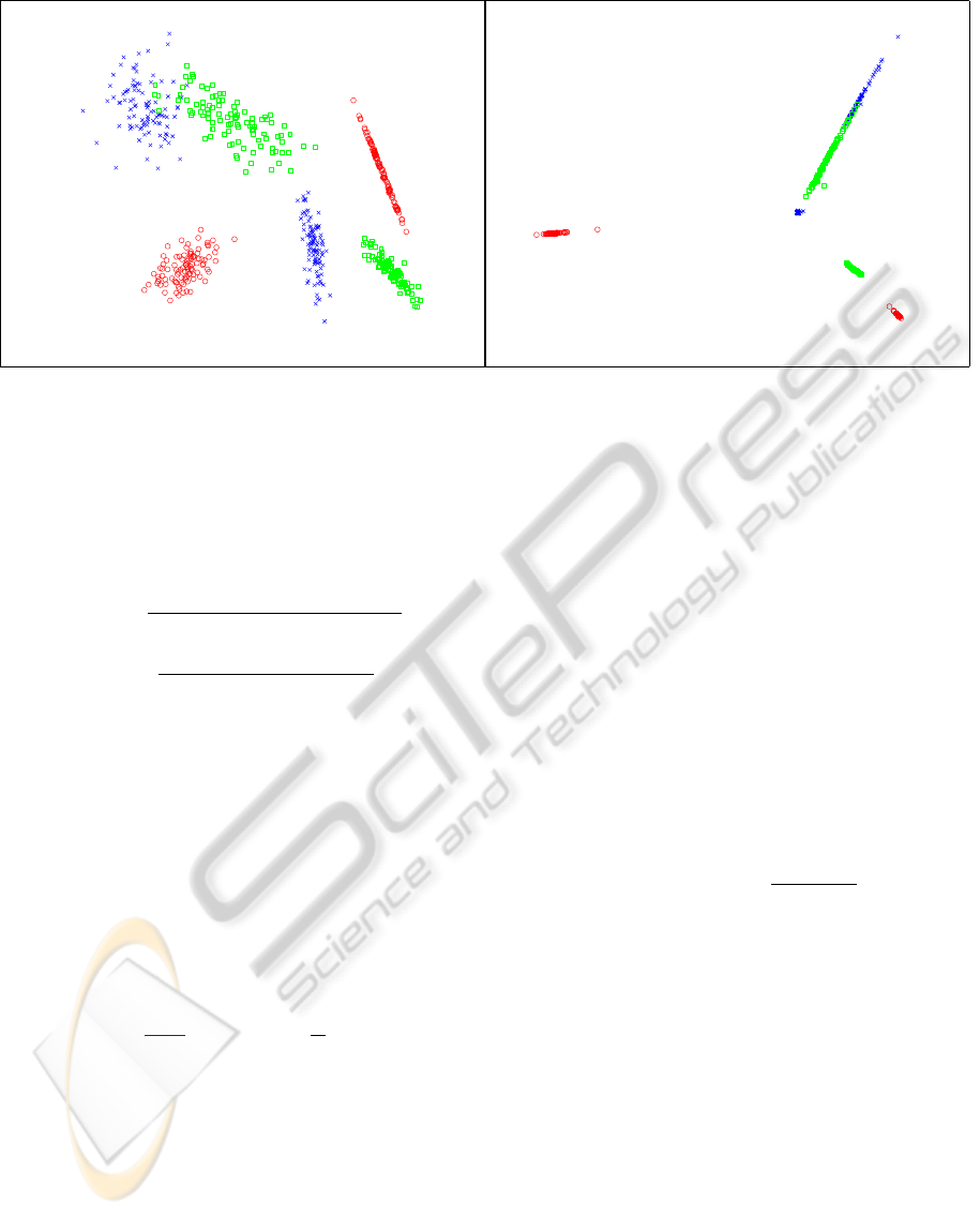
Figure 1: A simple example which demonstrates important properties of the Fisher Riemannian tensor: multi-modality as
well as class overlaps are preserved. The original data are displayed at the left, a plot of the data equipped with the Fisher
metric displayed using metric multidimensional scaling is shown on the right, the arrows point to regions of overlap of the
classes, which are preserved by the metric.
where
b(x,c) = E
ξ(i|x,c)
{x
i
} − E
ξ(i|x)
{x
i
}
ξ(i|x,c) =
δ
c,c
i
exp(−kx − x
i
k
2
/2σ
2
)
∑
j
δ
c,c
j
exp(−kx − x
j
k
2
/2σ
2
)
ξ(i|x) =
exp(−kx − x
i
k
2
/2σ
2
)
∑
j
exp(−kx − x
j
k
2
/2σ
2
)
E denotes the empirical expectation, i.e. weighted
sums with weights depicted in the subscripts. If large
data sets or out-of-sample extensions are dealt with,
a subset of the data only is usually sufficient for the
estimation of J(x).
There exist different ways to approximate the path
integrals based on the Fisher matrix as discussed in
(Peltonen et al., 2004). An efficient way which pre-
serves locally relevant information is offered by T -
approximations: T equidistant points on the line from
x
i
to x
j
are sampled, and the Riemannian distance on
the manifold is approximated by d
T
(x
i
,x
j
) =
T
∑
t=1
d
1
x
i
+
t − 1
T
(x
j
− x
i
),x
i
+
t
T
(x
j
− x
i
)
where d
1
(x
i
,x
j
) = (x
i
−x
j
)
T
J(x
i
)(x
i
−x
j
) is the stan-
dard distance as evaluated in the tangent space of x
i
.
Locally, this approximation gives good results such
that a faithful dimensionality reduction of data can be
based thereon.
Now the question occurs what are benefits of an
integration of such knowledge. Here we present two
potential applications. Thereby, we restrict to one typ-
ical real-life benchmark data set, the USPS data, only
due to space limitations, results for alternative bench-
marks being similar.
3 APPLICATION (I): TRAINING A
VISUALIZATION MAPPING
Similar to many other nonlinear projection tech-
niques, t-SNE has the severe drawback that it scales
quadratically with the size of the training set making
it infeasible for large data sets. In addition, it does
not provide an explicit mapping of the points; rather,
out-of-sample extensions have to be implemented by
means of an additional optimization. Because of this
fact, it has been proposed in (Gisbrecht et al., 2013)
to extend t-SNE towards a mapping in the following
way: an explicit functional form is defined as
x 7→ y(x) =
∑
j
α
j
·
k(x, x
j
)
∑
l
k(x, x
l
)
where α
j
∈ Y are points in the projection space and
the points x
j
are taken from a fixed sample of data
points used to train the mapping. k is the Gaussian
kernel. This mapping is parameterized by α
j
. Due
to its form as a generalized linear mapping, these pa-
rameters can analytically be determined as the least
squares solution of an exemplary set of points x
i
and
projections y
i
obtained by standard t-SNE (or any
other dimensionality reduction technique). Then the
matrix A of parameters α
j
is given by
A = Y · K
−1
where K is the normalized matrix with entries
k(x
i
,x
j
)/
∑
j
k(x
i
,x
j
). Y denotes the matrix of pro-
jections y
i
, and K
−1
refers to the pseudo-inverse.
This technology, referred to as kernel t-SNE, has
the benefit that training can be done on a small sub-
ICPRAM2013-InternationalConferenceonPatternRecognitionApplicationsandMethods
36

set of data only, extending the mapping to the full
data set by means of the explicit mapping prescrip-
tion. Thus, a considerable speed up can be obtained,
provided a small subsample of points is sufficient to
train the mapping. However, here occurs a problem:
often, the structure of the data such as clusters is not
yet pronounced if only a small sample of data is used
for training kernel t-SNE. In consequence, kernel t-
SNE when trained on a subsample does not clearly
emphasize an underlying class structure as compared
to t-SNE when trained on the full data set.
Here, discriminative dimensionality reduction of-
fers a possibility to substitute the loss of information
due to a small training set by prior information as
given by an explicit class labeling. On the one hand, it
is possible to generate the training set of points x
i
and
its projections y
i
for kernel t-SNE based on the Fisher
metric provided class labeling c
i
is available. In addi-
tion, kernel t-SNE can be extended to a discriminative
mapping by using the Fisher metric also in the kernel
mapping prescription k(x, x
j
).
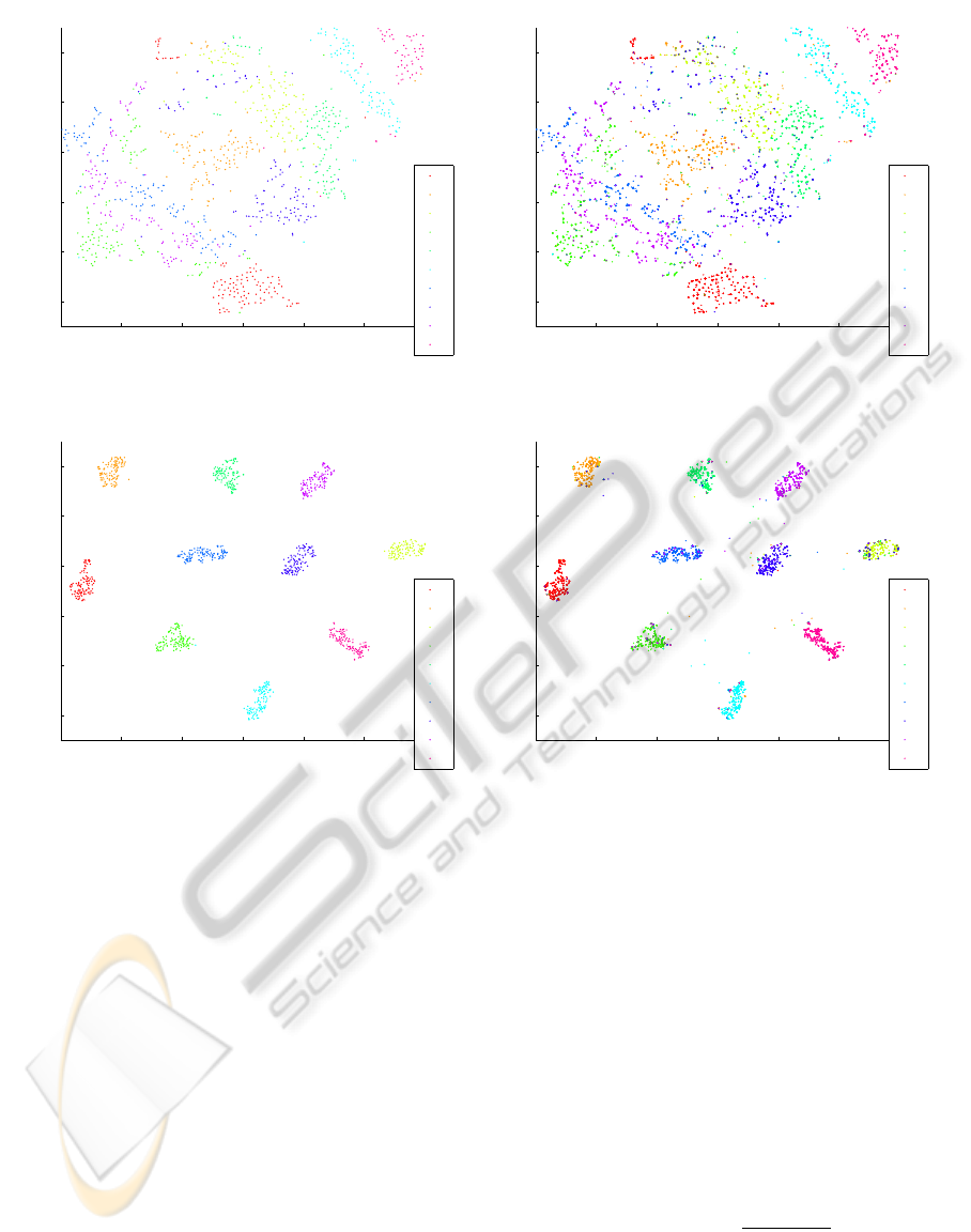
Fig. 2 and Fig. 3 show example mappings of the
USPS data set consisting of 11.000 points with 256
dimensions representing handwritten digits from 0 to
9 (Hastie et al., 2001). For training and the representa-
tion of the kernel mapping, 10% of the data are used.
For the estimation of the Fisher information, 1% of
the data are used. Clearly, the original kernel t-SNE
mapping does not contain enough information to em-
phasize the cluster structure when trained on 10% of
the data only, while t-SNE when trained on the full
data set clearly displays the classes, as can be seen
e.g. in (Maaten and Hinton, 2008). The resulting ker-
nel t-SNE mapping and its out of sample extension
are displayed in Fig. 2. In contrast, the cluster struc-
ture is clearly visible if auxiliary information is taken
into account, Fisher kernel t-SNE and its extension to
the full data set being displayed in Fig. 3.
4 APPLICATION (II):
VISUALIZATION OF
CLASSIFIERS
Classification constitutes one of the standard tasks in
data analysis. At present, the major way to display
the result of a classifier and to judge its suitability is
by means of the classification accuracy. Visualization
is used in only a few places when inspecting a clas-
sifier: If data live in a low dimensional space, a di-
rect visualization of the data points and classification
boundaries in 2D or 3D can be done. For high dimen-
sional data, which constitutes the standard case, a di-
rect visualization of the classifier is not possible. One
line of research addresses visualization techniques to
accompany the accuracy by an intuitive interface to
set certain parameters of the classification procedure,
such as e.g. ROC curves to set the desired speci-
ficity, or more general interfaces to optimize param-
eters connected to the accuracy (Hernandez-Orallo
et al., 2011). Surprisingly, there exists relatively lit-
tle work to visualize the underlying classifier itself
for high dimensional settings. For the popular sup-
port vector machine, for examples, only some specific
approaches have been proposed: one possibility is to
let the user decide an appropriate linear projection di-
mension by means of tour methods (Caragea et al.,
2008). As an alternative, some techniques rely on
the distance of the data points to the class boundary
and present this information using e.g. nomograms
(Jakulin et al., 2005) or by using linear projection
techniques on top of this distance (Poulet, 2005). A
few nonlinear techniques exist such as SVMV (Wang
et al., 2006), which visualizes the given data by means
of a self-organizing map and displays the class bound-
aries by means of sampling. Further, very interesting
nonlinear dimensionality reduction, albeit not for the
primary aim of classifier visualization, has been in-
troduced in (Braun et al., 2008). These techniques
offer first steps to visually inspect an SVM solution
such that the user can judge e.g. remaining error re-
gions, the modes of the given classes, outliers, or the
smoothness of the separation boundary based on a vi-
sual impression.
However, so far, these techniques are often only
linear, they require additional parameters, and they
provide combinations of a very specific classifier such
as SVM and a specific visualization technique. Dis-
criminative dimensionality reduction constitutes an
important technique based on which a given classi-
fier can be visualized. Here, we propose a princi-
pled alternative based on discriminative t-SNE with
the Fisher metric. We assume a classification map-
ping f : X → {1, ..., c} is present, which can be given
by a support vector machine, for example. This map-
ping has been trained using some points x
i
and their
label c
i
. We assume that the label prediction f (x
i
)
of a point x
i
can be accompanied by a real value
r(x
i
) ∈ R which indicates the (signed) strength of
class-membership association. This can be given by
the class probability or the distance from the decision
boundary, for example. Now the task is to map the
data points x
i
as well as the classification boundary
induced by f to two dimensions.
A very simple approach consists in a sampling of
the original space X and a projection of these data
x colored by class labels f (x) using a standard di-
ApplicationsofDiscriminativeDimensionalityReduction
37
−60 −40 −20 0 20 40 60
−60
−40
−20
0
20
40
1
2
3
4
5
6
7
8
9
0
−60 −40 −20 0 20 40 60
−60
−40
−20
0
20
40
1
2
3
4
5
6
7
8
9
0
Figure 2: Visualization of the USPS data set using kernel t-SNE for the training set (top) and out of sample extension (bottom).
−60 −40 −20 0 20 40 60
−60
−40
−20
0
20
40
1
2
3
4
5
6
7
8
9
0
−60 −40 −20 0 20 40 60
−60
−40
−20
0
20
40
1
2
3
4
5
6
7
8
9
0
Figure 3: Visualization of the USPS data set using discriminative Fisher kernel t-SNE for the training set (left) and out of
sample extension (right). Fisher kernel t-SNE provides clear class structures on these data unlike simple kernel t-SNE.
mensionality reduction technique. Since smooth val-
ues r(x) are present, isobars corresponding to the
classifier can then be displayed in the plane. This
naive approach encounters two problems: (i) sam-
pling the original data space X is infeasible due to
a usually high dimensionality and (ii) projecting ex-
haustive samples from high dimensions to 2D neces-
sarily encounters loss of possibly relevant informa-
tion.
These two problems can be avoided if label infor-
mation is taken into account already at the dimension-
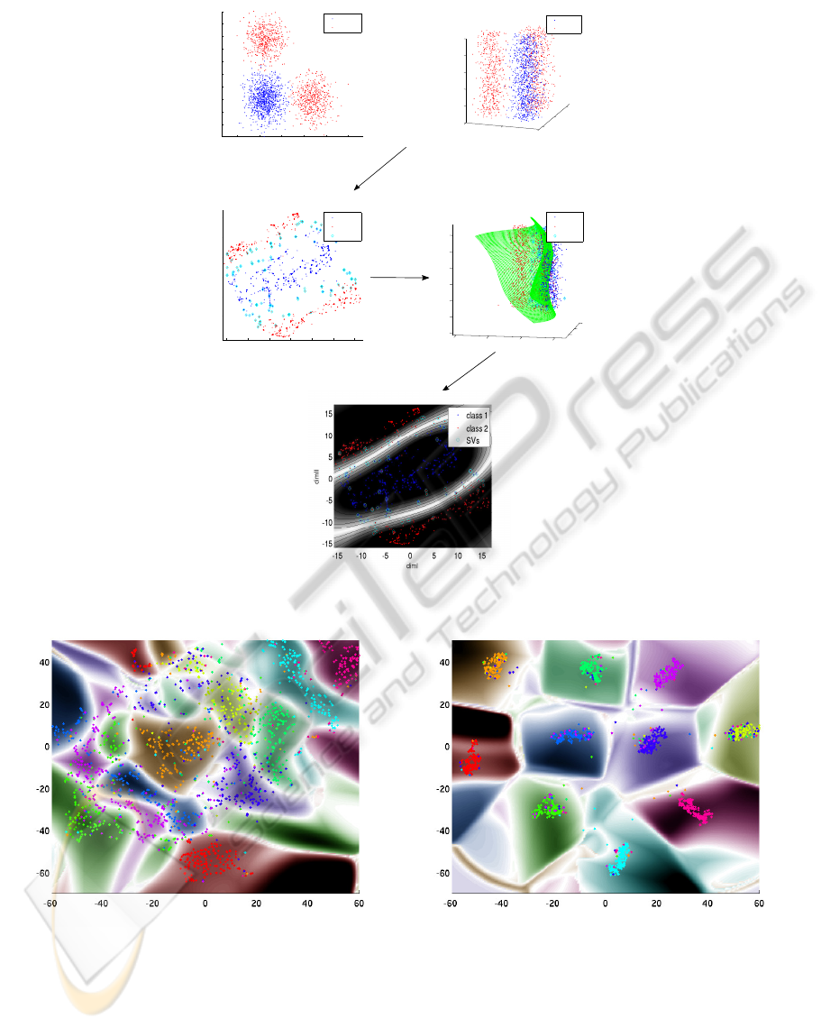
ality reduction step. We propose the following proce-
dure as displayed in Fig. 4:
• Project the data x
i
using a nonlinear discrimi-
native visualization technique leading to points
p(x
i
) ∈ Y = R
2
.
• Sample the projection space Y leading to points
z
0
i
. Determine points z
i
in the data space X which
are projected to these points p(z
i
) ≈ z
0
i
.
• Visualize the training points x
i
together with
the contours induced by the sampled function
(z
0
i
,r(z
i
)).
This procedure avoids the problems of the naive ap-
proach: on the one hand, a discriminative dimen-
sionality reduction technique focusses on the aspects
which are particularly relevant for the class labels and
thus emphasizes the important characteristics of the
classification function. On the other hand, sampling
takes place in the projection space only, which is low
dimensional.
One question remains: how can we find points z
i
∈
X which correpond to the projections z
0
i
∈ Y ? For this
purpose, we take an approach similar to kernel t-SNE:
we define a mapping
p
−1
: Y → X,y 7→
∑
i
α
i
·
k
i
(y
i
,y)
∑
i
k
i
(y
i
,y)
= A · [K]
i
of the projection space to the original space which is
trained based on the given samples x
i
, its projections
y
i
, and its labels c
i
. As before, k is the Gaussian ker-
nel, K the kernel matrix applied to the points y
i
which
ICPRAM2013-InternationalConferenceonPatternRecognitionApplicationsandMethods
38
0 0.2 0.4 0.6 0.8 1
0
0.1
0.2
0.3
0.4
0.5
0.6
0.7
0.8
0.9
1
dim1
dim2
class 1
class 2
class 2
0
0.5
1
0
0.5
1
0
0.2
0.4
0.6
0.8
1
dim1
dim2
dim3
class 1
class 2
0
0.5
1
1.5
0
0.5
1
−0.2
0
0.2
0.4
0.6
0.8
1
dim2
dim1
dim3
class 1
class 2
SVs
train classifier
project data down
−15 −10 −5 0 5 10 15
−15
−10
−5
0
5
10
15
dimI
dimII
class 1
class 2
SVs
sample
project up
classify
Figure 4: Principled procedure how to visualize a given data set and a trained classifier. The example displays a SVM trained
in 3D.
Figure 5: Visualization of an SVM classifier trained on the USPS data set by means of kernel t-SNE (top) and Fisher kernel
t-SNE (bottom).
are projections of x
i
and [K]
i
the ith column. A is
the matrix of parameters α
i
. These parameters α
i
are
determined by means of a numeric optimization tech-
nique such that the following error is minimized:
λ
1
· kX − A · Kk
2
+ λ
2
· kr(X) − r(A · K)k
2
Thereby, X denotes the points x
i
used to train the
discriminative mapping. r(·) denotes real values asso-
ciated to the classification f indicating the strength of
the class-membership association. λ
1
and λ
2
are posi-
tive weights which balance the two objectives formal-
ized by this functional form: a correct inverse map-
ping of the data x
i
and its projections y
i
on the one
side and a correct match of the induced classifications
via the given classifier f on the other side.
ApplicationsofDiscriminativeDimensionalityReduction
39

An example application of this procedure for the
USPS data set is based on the k t-SNE projections as
specified in the last paragraph. An SVM with Gaus-
sian kernel is trained on a subset of the data which
is not used to train the subsequent kernel t-SNE or
Fisher kernel t-SNE, respectively. A classification ac-
curacy of 99% on the training set and 97% on the test
set arises. We use two different kernel t-SNE map-
pings to obtain a training set for the inverse mapping
p
−1
: kernel t-SNE and Fisher kernel t-SNE, respec-
tively. The weights of the cost function has been cho-
sen as λ
1
= 0.1 and λ
2
= 10000, respectively. The re-
sulting visualization of the SVM classification is dis-
played in Fig. 5(top) if the procedure is based on ker-
nel t-SNE and Fig. 5(bottom) if the procedure is based
on Fisher kernel t-SNE.
Obviously, the visualization based on Fisher ker-
nel t-SNE displays much clearer class boundaries as
compared to a visualization which does not take the
class labeling into account. This visual impression is
mirrored by a quantitative comparison of the projec-
tions. For the kernel t-SNE mapping, the classifica-
tion induced in 2D as displayed in the map coincides
with the original classification with a 85% accuracy
only. If Fisher kernel t-SNE is used, the coincidence
increases to 92%.
5 CONCLUSIONS
We have reviewed discriminative dimensionality re-
duction, its link to the Fisher information matrix, and
we have discussed its difference to a direct classifica-
tion. Based on Fisher kernel t-SNE, two applications
have been proposed: a speed-up of dimensionality re-
duction on the one side and a visualization of a classi-
fier such as SVM on the other side. So far, the appli-
cations have been demonstrated using one benchmark
only, results for alternative benchmarks being similar.
Note that the proposed techniques are not restricted
to t-SNE, rather, similar techniques could be based on
top of popular alternatives such as LLE or Isomap.
ACKNOWLEDGEMENTS
Funding by DFG under grants number HA 2719/7-1,
HA 2719/4-1 and by the CITEC centre of excellence
are gratefully acknowledged. We would like to thank
the anonymous reviewers for helpful comments and
suggestions.
REFERENCES
Baudat, G. and Anouar, F. (2000). Generalized discriminant
analysis using a kernel approach. Neural Computa-
tion, 12:2385–2404.
Bekkerman, R., Bilenko, M., and Langford, J., editors
(2011). Scaling up Machine Learning. Cambridge
University Press.
Biehl, M., Hammer, B., Mer
´
enyi, E., Sperduti, A., and
Villmann, T., editors (2011). Learning in the con-
text of very high dimensional data (Dagstuhl Seminar
11341), volume 1.
Braun, M. L., Buhmann, J. M., and M
¨
uller, K.-R. (2008).
On relevant dimensions in kernel feature spaces. J.
Mach. Learn. Res., 9:1875–1908.
Bunte, K., Biehl, M., and Hammer, B. (2012a). A general
framework for dimensionality reducing data visualiza-
tion mapping. Neural Computation, 24(3):771–804.
Bunte, K., Schneider, P., Hammer, B., Schleif, F.-M., Vill-
mann, T., and Biehl, M. (2012b). Limited rank matrix
learning, discriminative dimension reduction and vi-
sualization. Neural Networks, 26:159–173.
Caragea, D., Cook, D., Wickham, H., and Honavar, V.
(2008). Visual methods for examining svm classi-
fiers. In Simoff, S. J., B
¨
ohlen, M. H., and Mazeika, A.,
editors, Visual Data Mining, volume 4404 of Lecture
Notes in Computer Science, pages 136–153. Springer.
Cohn, D. (2003). Informed projections. In Becker, S.,
Thrun, S., and Obermayer, K., editors, NIPS, pages
849–856. MIT Press.
Geng, X., Zhan, D.-C., and Zhou, Z.-H. (2005). Supervised
nonlinear dimensionality reduction for visualization
and classification. IEEE Transactions on Systems,
Man, and Cybernetics, Part B, 35(6):1098–1107.
Gisbrecht, A., Mokbel, B., and Hammer, B. (2013). Linear
basis-function t-sne for fast nonlinear dimensionality
reduction. In IJCNN.
Goldberger, J., Roweis, S., Hinton, G., and Salakhutdinov,
R. (2004). Neighbourhood components analysis. In
Advances in Neural Information Processing Systems
17, pages 513–520. MIT Press.
Hastie, T., Tibshirani, R., and Friedman, J. (2001). The
Elements of Statistical Learning. Springer Series in
Statistics. Springer New York Inc., New York, NY,
USA.
Hernandez-Orallo, J., Flach, P., and Ferri, C. (2011). Brier
curves: a new cost-based visualisation of classifier
performance. In International Conference on Machine
Learning.
Iwata, T., Saito, K., Ueda, N., Stromsten, S., Griffiths,
T. L., and Tenenbaum, J. B. (2007). Parametric em-
bedding for class visualization. Neural Computation,
19(9):2536–2556.
Jakulin, A., Mo
ˇ
zina, M., Dem
ˇ
sar, J., Bratko, I., and Zu-
pan, B. (2005). Nomograms for visualizing support
vector machines. In Proceedings of the eleventh ACM
SIGKDD international conference on Knowledge dis-
covery in data mining, KDD ’05, pages 108–117, New
York, NY, USA. ACM.
ICPRAM2013-InternationalConferenceonPatternRecognitionApplicationsandMethods
40

Kaski, S., Sinkkonen, J., and Peltonen, J. (2001).
Bankruptcy analysis with self-organizing maps in
learning metrics. IEEE Transactions on Neural Net-
works, 12:936–947.
Lee, J. A. and Verleysen, M. (2007). Nonlinear dimension-
ality reduction. Springer.
Lee, J. A. and Verleysen, M. (2010). Scale-independent
quality criteria for dimensionality reduction. Pattern
Recognition Letters, 31:2248–2257.
Ma, B., Qu, H., and Wong, H. (2007). Kernel clustering-
based discriminant analysis. Pattern Recognition,
40(1):324–327.
Maaten, L. V. D. and Hinton, G. (2008). Visualizing high-
dimensional data using t-sne. Journal of Machine
Learning Research, 9:2579–2605.
Memisevic, R. and Hinton, G. (2005). Multiple relational
embedding. In Saul, L. K., Weiss, Y., and Bottou, L.,
editors, Advances in Neural Information Processing
Systems 17, pages 913–920. MIT Press, Cambridge,
MA.
Mika, S., R
¨
atsch, G., Weston, J., Sch
¨
olkopf, B., and M
¨
uller,
K.-R. (1999). Fisher discriminant analysis with ker-
nels. In Neural Networks for Signal Processing IX,
1999. Proceedings of the 1999 IEEE Signal Process-
ing Society Workshop, pages 41–48. IEEE.
Peltonen, J., Klami, A., and Kaski, S. (2004). Improved
learning of riemannian metrics for exploratory analy-
sis. Neural Networks, 17:1087–1100.
Poulet, F. (2005). Visual svm. In Chen, C.-S., Filipe, J.,
Seruca, I., and Cordeiro, J., editors, ICEIS (2), pages
309–314.
R
¨
uping, S. (2006). Learning Interpretable Models. PhD
thesis, Dortmund University.
Tsang, I. W., Kwok, J. T., ming Cheung, P., and Cristianini,
N. (2005). Core vector machines: Fast svm training
on very large data sets. Journal of Machine Learning
Research, 6:363–392.
Vellido, A., Martin-Guerroro, J., and Lisboa, P. (2012).
Making machine learning models interpretable. In
ESANN’12.
Venna, J., Peltonen, J., Nybo, K., Aidos, H., and Kaski, S.
(2010). Information retrieval perspective to nonlinear
dimensionality reduction for data visualization. Jour-
nal of Machine Learning Research, 11:451–490.
Wang, X., Wu, S., Wang, X., and Li, Q. (2006). Svmv -
a novel algorithm for the visualization of svm classi-
fication results. In Wang, J., Yi, Z., Zurada, J., Lu,
B.-L., and Yin, H., editors, Advances in Neural Net-
works - ISNN 2006, volume 3971 of Lecture Notes in
Computer Science, pages 968–973. Springer Berlin /
Heidelberg.
Ward, M., Grinstein, G., and Keim, D. A. (2010). Interac-
tive Data Visualization: Foundations, Techniques, and
Application. A. K. Peters, Ltd.
Witten, D. M. and Tibshirani, R. (2011). Supervised mul-
tidimensional scaling for visualization, classification,
and bipartite ranking. Computational Statistics and
Data Analysis, 55(1):789 – 801.
ApplicationsofDiscriminativeDimensionalityReduction
41
