
Automatic Feature Selection for Sleep/Wake Classification
with Small Data Sets
J. Foussier
1
, P. Fonseca
2
, X. Long
2
and S. Leonhardt
1
1
Philips Chair for Medical Information Technology, RWTH Aachen University, Pauwelsstrasse 20, 52074 Aachen, Germany
2
Philips Research Eindhoven, High Tech Campus 34, 5656AE Eindhoven, The Netherlands
Keywords:
Sleep Monitoring, Sleep Staging, Feature Selection, Linear Discriminant Classification, Unobtrusive Moni-
toring, Cohen’s Kappa, Spearman’s Ranked-order Correlation.
Abstract:
This paper describes an automatic feature selection algorithm integrated into a classification framework devel-
oped to discriminate between sleep and wake states during the night. The feature selection algorithm proposed
in this paper uses the Mahalanobis distance and the Spearman’s ranked-order correlation as selection criteria to
restrict search in a large feature space. The algorithm was tested using a leave-one-subject-out cross-validation
procedure on 15 single-night PSG recordings of healthy sleepers and then compared to the results of a standard
Sequential Forward Search (SFS) algorithm. It achieved comparable performance in terms of Cohen’s kappa
(κ = 0.62) and the Area under the Precision-Recall curve (AUC
PR
= 0.59), but gave a significant computational
time improvement by a factor of nearly 10. The feature selection procedure, applied on each iteration of the
cross-validation, was found to be stable, consistently selecting a similar list of features. It selected an average
of 10.33 features per iteration, nearly half of the 21 features selected by SFS. In addition, learning curves
show that the training and testing performances converge faster than for SFS and that the final training-testing
performance difference is smaller, suggesting that the new algorithm is more adequate for data sets with a
small number of subjects.
1 INTRODUCTION
Sleep is an essential process in most animals, includ-
ing human beings, and although it has been stud-
ied for centuries, relatively little is known about it.
It is clear, however, that sleep is essential to sur-
vive, as sleep deprivation studies on rats have shown
(Rechtschaffen and Bergmann, 1995). Computer-
aided sleep assessment was introduced to reduce the
manpower and costs needed to collect and interpret
data during these studies. However, most of these
systems still require the subjects to spend one or
more nights in a sleep laboratory, which remains a
rather expensive and inconvenient procedure. Ambu-
latory sleep monitoring aims precisely at eliminating
this requirement and can effectively be used for di-
agnosing several sleep disorders. For this, new sen-
sors and algorithms are needed. Significant work has
been done to exploit the fact that certain autonomic
changes associated with different sleep stages also
manifest themselves differently in parameters such as
cardiorespiratory activity and body movements. By
evaluating how these parameters change, it should be
possible, at least to a certain extent, to distinguish
some of these stages without resorting to EEG. Sev-
eral research groups have worked on the extraction of
cardiorespiratory and body movement features (e.g.,
(Devot et al., 2007), (Devot et al., 2010), (Redmond
et al., 2007) or (Zoubek et al., 2007)). However, one
of the main issues is that many publications address
the sleep stage classification problem from a rather
limited set of physiological features. Many authors
report how successful a certain feature is for the clas-
sification task, instead of focusing on methods that
aim at selecting the best set of features as we will
show later. There is, in fact, a plethora of features
described in literature which can be readily used for
the task of sleep staging or the extraction of relevant
sleep parameters.
Most available PSG data were generated for pa-
tients with sleep disorders. As a result, prior work
related to sleep staging of healthy subjects with car-
diorespiratory signals or actigraphy often relies on
very small data sets (often less than a dozen subjects)
and were collected by individual research groups
for the validation of a new sensor and/or feature.
178
Foussier J., Fonseca P., Long X. and Leonhardt S..
Automatic Feature Selection for Sleep/Wake Classification with Small Data Sets.
DOI: 10.5220/0004245401780184
In Proceedings of the International Conference on Bioinformatics Models, Methods and Algorithms (BIOINFORMATICS-2013), pages 178-184
ISBN: 978-989-8565-35-8
Copyright
c
2013 SCITEPRESS (Science and Technology Publications, Lda.)

Many authors opt to perform a single feature selec-
tion step on the entire data set when applying tra-
ditional machine learning approaches, clearly bias-
ing the classification results towards positive per-
formance. Also, each single epoch is subject- and
time-dependent. Therefore the data of several sub-
jects cannot be (randomly) mixed and tested in a tra-
ditional leave-one-out-cross-validation (LOOCV) but
rather with a leave-one-subject-out-cross-validation
(LOSOCV) procedure, which reduces the number of
possible folds in the cross-validation.
Finding the ideal set of features for sleep/wake
classification, especially for small data sets, is a com-
plex and challenging task especially when the number
of features is large. An exhaustive search, although
leading to the optimal feature set, is impractical in
terms of computational time as soon as the dimen-
sion of the feature space becomes larger. Sequential
search, backward (SBS) and forward (SFS), tries to
address this issue by following a single search path
during the process (Whitney, 1971). However, it often
delivers sub-optimal solutions especially in problems
with small data sets. In the work of (Zoubek et al.,
2007) an example of the employment of the SFS al-
gorithm can be found.
Building upon previous research published by
(Devot et al., 2007; Devot et al., 2010), we will de-
scribe a new feature selection method that is particu-
larly adequate for use in each single training step of
the LOSOCV and for linear discriminant classifiers.
Linear discriminant classifiers, like most other clas-
sifiers, are sensitive to the dimension of the feature
space. A large number of features can also cause
over-fitting and prevent the classifier from general-
izing well to new data when assuming a certain de-
gree of independence between the features. On the
other hand, if the dimension is too small the classi-
fier will often be too sensitive to noise (Duda et al.,
2001). Computational time also plays a role, es-
pecially when the number of available features in-
creases. All these constraints have been taken into
account during the design process of the feature se-
lection algorithm. In addition, as we will show, this
feature selection method is also well suited for data
sets with small number of subjects. Finally, by inte-
grating feature selection in the training step of a cross-
validation procedure, we will guarantee that the train-
ing (including feature selection) and testing steps are
performed on mutually exclusive data sets, and at the
same time on the largest possible data set. We will
then apply and evaluate the proposed feature selec-
tion method within a classification framework used
for sleep/wake detection in healthy sleepers. In or-
der to highlight the properties of the proposed feature
selection algorithm, all classification results, includ-
ing total computational time, stability of the selected
features and generalization capabilities, are compared
to a standard Sequential Forward Search (SFS) algo-
rithm.
2 METHODS AND MATERIALS
2.1 Data Set
The data set consists of 15 single-night PSG
recordings of healthy sleepers – ten female
(age 31±12.4 yrs, BMI 24.76±3.7 kg/m
2
)
and five male subjects (age 31±5.5 yrs,
BMI 24.38±2.72 kg/m
2
). Each PSG recording
includes at least the EEG channels recommended by
the American Academy of Sleep Medicine (AASM),
a 2-lead ECG and the thoracic respiratory effort.
In addition, actigraphy was acquired with a Philips
Actiwatch and synchronized with the PSG. Nine
subjects were measured in Boston (USA), at the
Sleep Health Center, and six subjects in Eindhoven
(The Netherlands), at the sleep laboratory of the High
Tech Campus. The study protocol was approved by
the Ethics Committees of the respective center and
all subjects signed an informed consent form. Sleep
stages were scored by professional sleep technicians
according to the guidelines of the AASM as wake,
non-REM sleep 1-3 (N1-N3) and REM sleep using
30-second epochs. In order to train and test our
classifier for the sleep and wake classes, we merged
the N1-N3 and REM classes into a single sleep class.
Since the data were recorded in two different sleep
laboratories, with two differently configured PSG sys-
tems, the data were first resampled to a common sam-
pling rate (512 Hz for ECG, 10 Hz for respiratory ef-
fort, and 30-second period for actigraphy).
2.2 Classification Framework
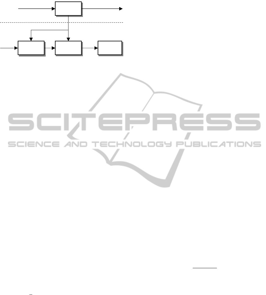
The classification framework, illustrated in Figure 1,
is divided in two main parts: training and classifica-
tion. Before training, the data set is first split into
independent training and testing sets. Each contains
manually annotated sleep scores, indicating the sleep
stage for every epoch. The predictions of the classi-
fier are compared with the ground-truth annotations
and the performance of the classifier on the testing set
is computed.
As mentioned in the introduction, autonomic
changes associated with different sleep stages will
manifest themselves differently in certain physiolog-
ical parameters. In order to exploit these changes we
AutomaticFeatureSelectionforSleep/WakeClassificationwithSmallDataSets
179
Feature subset
selection
Classification Evaluation
Training data
Feature
selection and
training
Feature short-list
and model
P
r
e
d
i
c
t
i
o
n
s
Selected features
Testing
data
Training
Classification
Model
Figure 1: Block diagram illustrating the classification
framework.
extracted a total of 60 features from the ECG, the res-
piratory (thoracic) effort and the actigraphy signals
on 30-second epochs. The cardiac features are based
on heart-rate-variability (HRV) evaluated in time and
frequency domain. Non-linear properties were also
examined based on Detrended Fluctuation Analysis
(DFA) and Sample Entropy. The respiratory features
were defined in the time domain - including statistical
measures derived from both the signal waveform and
respiratory period and non-linear measures of “simi-
larity” - as well as in the frequency domain. For actig-
raphy, we used so-called activity counts, directly ac-
quired with the Actiwatch. Since we did not put any
additional effort on the task of feature extraction, we
will not mention it further in this paper and refer to
previous work (Devot et al., 2010; Long et al., 2012).
The training step comprises an iterative feature
selection procedure whereby a short-list of features
of the original 60 features is chosen. This short-list
should comprise the set of features that best character-
izes the different sleep stages accordingly to the anno-
tations of the training set. On each iteration of feature
selection, the input feature vectors are reduced to a
subset of feature vectors. This subset is then used to
train a model which is in turn used to classify the same
input data. The training classification performance is
fed back to the feature selection procedure.
Assuming that all features are normally dis-
tributed and the covariance matrices for all classes are
identical, i.e., Σ
Σ
Σ
a
a
a
= Σ
Σ
Σ, we have a “linear discriminant”
function given by
g
a
(f) = −
1
2
(f − µ
µ
µ
a
a
a
)
0
Σ
Σ
Σ
−1
(f − µ
µ
µ
a
a
a
) + ln(P(ω
a
)) (1)
where µ
µ
µ
a
a
a
and Σ
Σ
Σ are the mean vector for class ω
a
and
the pooled covariance matrix (Duda et al., 2001; Red-
mond et al., 2007). To use this function in the train-
ing step of our classification framework, we need to
compute the sample mean and the prior probabilities
of each class and the inverse pooled covariance ma-
trix Σ
Σ
Σ. We chose the linear discriminant instead of
a quadratic discriminant, because quadratic discrim-
inants are known to require larger sample sizes than
linear discriminants and they also seem to be more
sensitive to possible violations of the basic assump-
tions of normality (Friedman, 2012). This is partic-
ularly important for classification of features derived
from physiological data, which very often do not fol-
low a normal distribution. Furthermore, for prob-
lems with small sample sizes it is also common to use
the pooled covariance estimate as a replacement of
the population class covariance matrices (Friedman,
2012).
Regarding the prior probabilities P (ω
a
) of each
class, we used the observation that the different
classes have different probabilities throughout the
night (Redmond et al., 2007). The time-dependent
prior probabilities for a given class can be obtained
by counting, for each epoch relative to the beginning
(i.e., when lights were turned off) of each recording,
the number of times that epoch was annotated with
that class. The prior probability term in the linear dis-
criminant (1) can be used to bias the classification to
a certain class.
The feature selection procedure described in this
paper aims at selecting features that simultaneously
offer a high discrimination power between classes, yet
are uncorrelated with each other. It makes use of the
classifier structure and theory. It can be shown that
when using the linear discriminant function in (1) in a
two-class problem where the classes are equiprobable
the error probability of the classifier depends on the
following metric
δ
2
= (µ
µ
µ
a
− µ
µ
µ
b
)
0
Σ
Σ
Σ
−1
(µ
µ
µ
a
− µ
µ
µ
b
). (2)
This metric, also called the Mahalanobis distance, re-
flects the “class separability” for a given feature set.
As such, it seems appropriate to measure the dis-
criminating power of each individual feature. When
evaluating a single feature k, the inter-class distance
between the classes ω
a
and ω
b
can be rewritten as
d
k
=
µ
k
a
− µ
k
b
σ
k
(3)
where µ
k
a
and µ
k
b
are the population means of each
class and σ
k
is the standard deviation of feature k. The
top-discriminating features are those with the highest
inter-class distance d
k
. As a measure of correlation
between features, the algorithm uses the Spearman’s
ranked-order correlation (Abdullah, 1990). This cor-
relation measure is particularly robust in the presence
of outliers, very common when measuring physiolog-
ical signs. Unlike the Pearson’s correlation, it does
not require a linear relation between the features to
express the correlation between them. As an example
of signals with high Spearman’s ranked-order and low
Pearson’s correlation, consider the inter-beat interval
BIOINFORMATICS2013-InternationalConferenceonBioinformaticsModels,MethodsandAlgorithms
180

(IBI) and the derived instantaneous heart rate (HR):
HR = IBI
−1
. It is clear that HR and IBI correlate
monotonically, but not linearly.
Maximum discrimination power and minimum
correlation are combined in the feature selection al-
gorithm described in the box on the right hand side
(“mahal”). The algorithm assigns a score to each fea-
ture (steps 1 to 4). The higher the score, the better a
feature is for our classification task. An iterative pro-
cedure will then search a variety of score thresholds,
and determine the classification performance obtained
with the corresponding feature short-list (step 5). The
highest performance will correspond to the optimal
short-list of features for our training set. Note that
when cross-validation is used to evaluate the perfor-
mance of a classifier, this procedure can be used with
the training set defined on each iteration. Each short-
list can then be used for classification with the testing
set of the same iteration.
Both the mahal and SFS feature selection meth-
ods will be evaluated by comparing the performance
in terms of κ and AUC
PR
on the training and the test-
ing set. Performance curves during the feature se-
lection procedure, learning curves and AUC
PR
val-
ues of the classification results using the selected fea-
tures of each cross-validation step, will all help giv-
ing us a good insight of the overall performance of
each feature selection method. In addition, the num-
ber and diversity of the selected features and the total
computation time are analyzed. It can be shown that
the fraction of misclassified epochs during LOSOCV
corresponds to the maximum likelihood estimate for
the (unknown) error rate of a classifier (Duda et al.,
2001). Although this procedure has also been used
to evaluate the performance of similar classifiers in
earlier work, the feature selection was applied on the
complete data set, and therefore, also on the testing
set. The feature selection described in this paper is
applied in each iteration of the LOSOCV, guarantee-
ing that the testing data used to validate the classi-
fier were not exposed to the tuning and training steps.
That means that for each iteration a separate short-list
of features is determined.
First, the performance of the classifier was evalu-
ated using the traditional metrics of accuracy, preci-
sion, specificity and sensitivity (considering wake as
the positive class) for each iteration of the LOSOCV
and for the pooled results (Fawcett, 2004). How-
ever, because the wake and sleep classes are very im-
balanced (the wake epochs represent less than 10%
of all epochs) these metrics can fail to give an ac-
curate overview of the performance for both classes
(Haibo and Garcia, 2009). For that reason we do not
present those metrics in this paper, but compute and
Algorithm 1: (mahal).
For the feature values and associated ground-truth
{
f
i
,y
i
}
of each epoch in a given training set:
Step 1
Compute the inter-class distance for each feature k as
d
k
=
f
k
a
− f
k
b
σ
k
(4a)
where the sample mean for a given class z and the standard
deviation are given by
f
k
z
=
∑
i∈Z
f
k
i
#Z
, for Z =
{
i|y
i
= z
}
(4b)
σ
k
=
v
u
u
u
t
N
∑
i=1
f
k
i
− f
k
2
N − 1
, with f
k
=
N
∑
i=1
f
k
i
N
(4c)
Collect all unique inter-class distances in an array d.
Step 2
Compute the Spearman’s ranked-order correlation c
k,l
between each feature and the remaining features
c
k,l
= corr
f
0
k
,f
0
l
(4d)
where f
0
k
and f
0
l
are the feature k and l respectively, for
each epoch in the training set.
Step 3
Assign a “score” s
k
of zero to each feature
s
k
:= 0, for k ∈
{
1,..., N
F
}
(4e)
Step 4
for each M in d and for C = 0...1, step size ∆
C
= 0.01
for each feature k
if d
k
> M and if the feature is uncorrelated
with the others,
c
k,l
< C,∀l ∈
{
1,..., N
F
}
(4f)
or has a higher distance than the feature it is
correlated with,
m
k
> m
l
,∀l ∈
l|l = 1, ...,N
F
,c
k,l
≥ C|
(4g)
increase its score
s
k
:= s
k
+
1
/N
S
(4h)
where N
S
is the number of loop steps,
N
S
=
#d
∆
C
(4i)
Step 5
for S = 0...1, step size ∆
S
=
1
/N
S
compile a short-list of features l
S
with score higher than
the threshold l
S
=
{
k|s
k
> S
}
, compute the performance
κ
S
of the classifier in the training set using l
S
.
Step 6
Return as the final short-list the list of features which gave
the highest performance l = l
S
MAX
, with
S
MAX
=
{
S|κ
S
= max (
{
κ
1
,κ
2
,...
}
)
}
. (4j)
AutomaticFeatureSelectionforSleep/WakeClassificationwithSmallDataSets
181
0 0.2 0.4 0.6 0.8 1
0.5
0.55
0.6
0.65
Cohen’s kappa (κ)
Score threshold
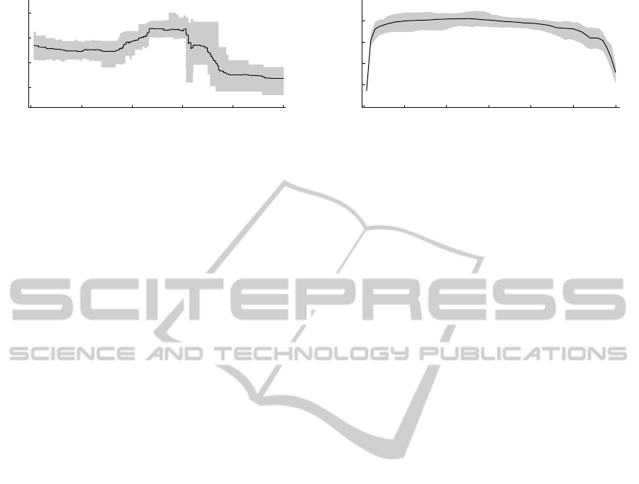
Figure 2: Performance κ on the training set for different
score thresholds.
analyze the Cohen’s Kappa coefficient of agreement
(κ) instead. This metric is directly interpretable as
the proportion of joint judgments for which there is
agreement, after chance agreement is excluded (Co-
hen, 1960). Despite their widespread use, these met-
rics only assess the classifier’s performance on a sin-
gle point in the entire solution space, namely that ob-
tained by directly comparing the output of the dis-
criminants defined for both classes by (1). To com-
pare a classifier with other classifiers this single point
might not be sufficient. By doing so, we assume
equal misclassification costs and fully known class
distributions (Provost et al., 1998). When there is
a large imbalance between the classes - as it is the
case for sleep/wake classification - Precision-Recall
(PR) curves should be used instead of Receiver Oper-
ating Characteristic (ROC) curves (Davis and Goad-
rich, 2006). In order to assess the performance of a
classifier across the entire solution space, it is custom-
ary to compute the area under the curve, in this case,
under the PR curve (AUC
PR
). Unlike the computation
of the AUC for the ROC curve, computing the AUC
for the PR curve requires a more complex procedure,
the composite trapezoidal method proposed by (Davis
and Goadrich, 2006).
Finally, we also computed so-called “learning
curves” (Duda et al., 2001) to gain insight into the
generalization capabilities of the classifier. By vary-
ing the number of subjects in the data set, these curves
can help predict what the performance of the classi-
fier would be when using more training data. They
can be obtained by computing the testing and training
error or alternatively, the testing and the training per-
formance (e.g., κ) for data subsets of different size n
randomly selected from the whole data set. As n in-
creases, the testing and training performance should
approach the same asymptotic value. The conver-
gence speed indicates how well a classifier is suited
for small data sets and has to be taken into account
when classifying small data sets.
0 10 20 30 40 50 60
0.5
0.55
0.6
0.65
0.7
Cohen’s kappa (κ)
Desired feature count
Figure 3: Performance κ on the training set for different
desired number of features in the SFS algorithm.
3 RESULTS
First, the performance κ obtained on the training set
for each score threshold S (step 5 of the feature se-
lection algorithm) is illustrated in Figure 2. To fur-
ther show the stability of the feature selection process,
we plotted with shaded bands the range between the
minimum and maximum κ obtained for each thresh-
old across all iterations of the LOSOCV. The perfor-
mance peaks around S = 0.5, with a relatively nar-
row shaded band. Intuitively, a narrow performance
band means that the performance obtained for a given
score threshold is similar across all iterations of the
LOSOCV, suggesting that the procedure is stable.
Note that with thresholds beyond 0.6, and therefore
with smaller short-lists, the performance drops. There
seems to be an optimal number of features which on
the one hand prevents overfitting while on the other
maximizes the generalization capabilities of our clas-
sifier. The use of a score threshold in this proce-
dure is advantageous since unlike many other feature
selection algorithms we do not need to specify the
“desired” number of features, letting that depend on
the actual properties of the training set. In a simi-
lar manner, by sweeping through a desired number
of features, we can observe how the performance of
SFS evolves (Figure 3). The average performance is
maximal when using 26 features. The width of the
shaded band is comparable to the one in Figure 2.
Note that the performance on the training set is higher
when compared with mahal, where from the begin-
ning more features correlated with each other, even
with high discriminative power, are excluded. This
typically leads to a higher performance on the train-
ing data set, but, as we will show, not necessarily on
the testing data set.
Table 1 lists the performance of the classifier on
the testing set for each iteration of the LOSOCV and
also the overall performance. The first column indi-
cates the iteration number of the LOSOCV. The three
columns with the headers mahal and SFS indicate the
BIOINFORMATICS2013-InternationalConferenceonBioinformaticsModels,MethodsandAlgorithms
182
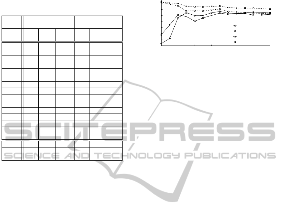
Table 1: Results on the testing set during cross-validation,
considering wake class as positive.
mahal SFS
(total time = 984 s) (total time = 9205 s)
it κ
κ
κ
AUC #
κ
κ
κ
AUC #
PR feat. PR feat.
1 0.77 0.83 8 0.77 0.85 20
2 0.58 0.73 7 0.70 0.75 15
3 0.66 0.61 7 0.71 0.77 21
4 0.55 0.82 10 0.65 0.89 31
5 0.61 0.80 15 0.67 0.68 31
6 0.94 0.94 7 0.73 0.92 17
7 0.76 0.85 16 0.69 0.78 24
8 0.89 0.93 10 0.81 0.86 22
9 0.76 0.89 8 0.63 0.88 27
10 0.28 0.28 11 0.32 0.32 17
11 0.70 0.79 10 0.71 0.77 21
12 0.60 0.83 9 0.64 0.74 11
13 0.56 0.68 14 0.68 0.76 10
14 0.24 0.35 13 0.49 0.59 30
15 0.53 0.80 10 0.58 0.80 18
pooled 0.62 0.59 - 0.64 0.60 -
mean 0.63 0.74 10.33 0.65 0.76 21
std 0.19 0.19 2.94 0.12 0.15 6.69
κ performance, the AUC
PR
and the number of selected
features for each iteration of the LOSOCV for the
mahal and the SFS algorithm, respectively. The row
pooled indicates the overall performance obtained af-
ter pooling all classification epochs. Note that this is
different from the average results, which are indicated
in the row mean with the standard deviation std. In
addition, the total computation time for all 15 feature
selection steps is included in the first row of the table.
Considering the classification performances com-
pared to the ground-truth, similar kappa values of 0.62
and 0.64 have been computed for mahal and SFS, re-
spectively. As it can also be seen, κ ranges from 0.24
to 0.94 for mahal and from 0.32 to 0.81 for SFS, re-
spectively. This shows that between-subject variation
is quite high, reflecting important physiological dif-
ferences between individuals, regardless of the em-
ployed feature selection algorithm. Also the AUC
PR
of both algorithms are comparable with 0.59 (mahal)
and 0.60 (SFS). A Wilcoxon signed rank test con-
firmed that the results are not significantly different
(p = 0.39).
Figure 4 displays the learning curves obtained
by varying the number of subjects in the data set.
The overall performances (pooled LOSOCV results)
achieved on the training and testing data sets with
mahal converge rapidly from 5 subjects and stabi-
lize around a κ of 0.65. SFS converges much slower.
The performance gap of κ between the training and
the testing remains higher than for mahal, even for
15 subjects. The performance on the training set re-
2 4 6 8 10 12 14
0.1
0.2
0.3
0.4
0.5
0.6
0.7
0.8
Number of subjects
Cohen’s kappa (κ)
training (mahal)
testing (mahal)
training (SFS)
testing (SFS)
Figure 4: Learning curves obtained by varying the number
of subjects in the training and testing sets.
mains slightly above 0.7, whereas the performance
for both mahal and SFS on the testing set are at
around 0.65.
4 DISCUSSION AND
CONCLUSIONS
The feature selection step, essential to the proper de-
sign of a good classifier, usually suffers from an im-
portant methodological issue: in the presence of little
available data, researchers often opt to perform fea-
ture selection on the complete data set. The feature se-
lection algorithm proposed in this paper addresses this
issue by offering the possibility of being integrated in
a cross-validation procedure. The algorithm is fully
automatic and, more importantly, does not require the
choice of a desired number of features.
Figure 2 and Figure 3 do not reflect how many
(different) features were chosen. Inspecting Table 1,
a big difference is noticeable in the number of se-
lected features. Where mahal selects about 10 fea-
tures in average, with standard deviation (std) of less
than 3 features, SFS selects 21 features with a stan-
dard deviation of nearly 7. The diversity of selected
features after selection with SFS is very high whereas
mahal consistently selects similar set of features dur-
ing the different iterations of the cross-validation pro-
cedure, also with one small data set. In order to
compare how consistently the feature selection algo-
rithms were across the different iterations of the cross-
validation procedure, we computed the mean number
(and standard deviation) of iterations each feature was
selected. The mahal algorithm chose 9.12 (5.42) and
SFS 6.43 (4.59) number of iterations per selected fea-
ture in average. Only 17 different features for mahal,
compared to 46 for SFS, were selected by the feature
selection process. Furthermore, each feature is se-
lected, in average, more times than with SFS which
further illustrates how stable the selection procedure
is to changes in the training set. A higher diversity of
features mainly has two drawbacks. First, it is more
difficult to choose a final set of features when design-
AutomaticFeatureSelectionforSleep/WakeClassificationwithSmallDataSets
183

ing a classifier, since this seems to vary with every
small change in the training set. Second, more fea-
tures means higher feature extraction time. Despite
the smaller number of selected features, the classifi-
cation performance was not significantly affected.
The performance of a feature selection algorithm
can also be described in terms of the total computa-
tional time that an algorithm needs to find the optimal
feature set. Here, we only analyze the time needed by
the feature selection itself. The feature extraction step
is not taken into account. mahal is nearly 10 times
faster than SFS, with 984 s and 9205 s, respectively.
By design, on each iteration SFS must redo the entire
classification step in the training set for each feature
before choosing which feature to add to the feature
set. The time increases approximately exponentially
with each new feature added to the total feature set.
In contrast, the computational time of the mahal algo-
rithm increases approximately linearly as the perfor-
mance calculations are only performed on the selected
feature subsets (step 5 of the algorithm). In addition,
the algorithm automatically restricts the list of fea-
tures that have to be tested during selection by eval-
uating their statistical power in advance, i.e., the Ma-
halanobis distance and the Spearman’s ranked-order
correlation.
Our classifier achieves a performance of κ = 0.62
in distinguishing sleep/wake, which is at least as high
as most work published so far, with fewer features
used during classification. However, the differences
in performance obtained for different subjects are too
large to be ignored. It seems from the learning curves
that this classifier is approaching its maximum per-
formance with the currently extracted features. In
order to further improve it, new approaches seem to
be needed. These could take into account, or bet-
ter yet, compensate for subject-specific differences
in the physiological expressions of different sleep
stages. Nevertheless, the feature selection algorithm
mahal described in this paper seems well-suited for
this problem since it is stable enough to be integrated
in a cross-validation procedure, also in the presence
of small data sets.
ACKNOWLEDGEMENTS
The authors thank Dr. Reinder Haakma and Sandrine
Devot, as well as Prof. Ronald Aarts for their com-
ments and careful reading of the manuscript.
REFERENCES
Abdullah, M. (1990). On a robust correlation coefficient.
The Statistician, 39(4):455–460.
Cohen, J. (1960). A Coefficient of Agreement for Nominal
Scales. Educational and Psychological Measurement,
20(1):37–46.
Davis, J. and Goadrich, M. (2006). The relationship
between Precision-Recall and ROC curves. In Pro-
ceedings of the 23rd international conference on Ma-
chine learning ICML 06, volume 10 of ICML ’06,
pages 233–240, Pittsburgh (USA). ACM Press.
Devot, S., Bianchi, A. M., Naujokat, E., Mendez, M.,
Brauers, A., and Cerutti, S. (2007). Sleep monitoring
through a textile recording system. In IEEE Engineer-
ing in Medicine and Biology Society, volume 2007,
pages 2560–2563.
Devot, S., Dratwa, R., and Naujokat, E. (2010). Sleep/wake
detection based on cardiorespiratory signals and actig-
raphy. In Annual International Conference of the
IEEE Engineering in Medicine and Biology Society
(EMBS), pages 5089–5092. IEEE.
Duda, R. O., Hart, P. E., and Stork, D. G. (2001). Pattern
Classification. Wiley, 2nd edition.
Fawcett, T. (2004). ROC Graphs: Notes and Practical Con-
siderations for Researchers. ReCALL, 31(HPL-2003-
4):1–38.
Friedman, J. H. (2012). Regularized Discriminant Analy-
sis. Journal of the American Statistical Association,
84(405):165–175.
Haibo, H. and Garcia, E. (2009). Learning from Imbalanced
Data. IEEE Transactions on Knowledge and Data En-
gineering, 21(9):1263–1284.
Long, X., Fonseca, P., Foussier, J., Haakma, R., and Aarts,
R. (2012). Using Dynamic Time Warping for Sleep
and Wake Discrimination. In IEEE Engineering in
Medicine and Biology Society - International Confer-
ence on Biomedical and Health Informatics (BHI),
volume 25, pages 886–889, Hong Kong/Shenzhen
(China).
Provost, F., Fawcett, T., and Kohavi, R. (1998). The case
against accuracy estimation for comparing induction
algorithms. In Proceedings of the 15th International
Conference on Machine Learning, volume 445. JS-
TOR.
Rechtschaffen, A. and Bergmann, B. (1995). Sleep depri-
vation in the rat by the disk-over-water method. Be-
havioural Brain Research, 69(1-2):55–63.
Redmond, S. J., de Chazal, P., O’Brien, C., Ryan, S., Mc-
Nicholas, W. T., and Heneghan, C. (2007). Sleep
staging using cardiorespiratory signals. Somnologie,
11(4):245–256.
Whitney, A. (1971). A Direct Method of Nonparametric
Measurement Selection. IEEE Transactions on Com-
puters, C-20(9):1100–1103.
Zoubek, L., Charbonnier, S., Lesecq, S., Buguet, A.,
and Chapotot, F. (2007). Feature selection for
sleep/wake stages classification using data driven
methods. Biomedical Signal Processing and Control,
2(3):171–179.
BIOINFORMATICS2013-InternationalConferenceonBioinformaticsModels,MethodsandAlgorithms
184
