ıve Bayes Domain Adaptation for Biological Sequences

Nic Herndon and Doina Caragea

Computing and Information Sciences, Kansas State University, 234 Nichols Hall, 66506, Manhattan, KS, U.S.A.

Keywords:

ıve Bayes, Domain Adaptation, Supervised Learning, Semi-supervised Learning, Self-training, Biological

Sequences, Protein Localization.

Abstract:

The increased volume of biological data requires automatic computation tools to analyze it. Although ma-

chine learning methods have been successfully used with biological sequences in a supervised framework,

their accuracy usually suffers when a classiﬁer is learned on a source domain and applied to a different, less

studied domain, in a domain adaptation framework. To address this issue, we propose to use an algorithm

that combines labeled sequences from a well studied organism, the source domain, with labeled and unlabeled

sequences from a related, less studied organism, the target domain. Our experimental results show that this

algorithm has high classifying accuracy on the target domain.

1 INTRODUCTION

The widespread use of next generation sequencing

(NGS) technologies in the recent years has resulted

in an increase in the volume of biological data gener-

ated, including both DNA sequences and also derived

protein sequences. A challenge arising from the in-

creased volume of data consists of the organization,

analysis, and interpretation of this data, in order to

create or improve genome assemblies or genome an-

notation, or to predict protein function, structure and

localization, among others. Some of these problems

can be framed as biological sequence classiﬁcation

problems, i.e., assigning one of several labels to a

DNA or protein sequence based on its content (e.g.,

predicting the presence or absence of an acceptor or

donor splice site in DNA sequences centered around

GT or AG dimers; or determining where a protein

is localized, such as in cytoplasm, inner membrane,

periplasm, outer membrane, or extracellular space,

a.k.a., protein localization).

Using machine learning or statistical inference

methods allows labeling of biological data several or-

ders of magnitude faster than it can be done manu-

ally, and with high accuracy. For example, hidden

Markov models are currently used in gene prediction

algorithms, and support vector machines have shown

promising results with handwritten digit classiﬁcation

(Vapnik, 1995), optical character recognition (M

uller

et al., 2001; Sch

olkopf and Smola, 2001) and transla-

tion initiation sites classiﬁcation based on proximity

to start codon within sequence window (M

uller et al.,

2001) or based on positional nucleotide incidences

(Zien et al., 2000), classiﬁcation into malign or be-

nign of gene expression proﬁles (Noble, 2006), ab ini-

tio gene prediction (Bernal et al., 2007), classiﬁcation

of DNA sequences into sequences with splice site at

a determined location or not (Jaakkola and Haussler,

1999; Sonnenburg et al., 2007; Tsuda et al., 2002;

Sonnenburg et al., 2002; Lorena and de Carvalho,

2003; R

atsch and Sonnenburg, 2004; Degroeve et al.,

2005; Huang et al., 2006; Zhang et al., 2006; Baten

et al., 2006), and classifying the function of genes

based on gene expression data (Brown et al., 2000).

However, using a supervised classiﬁer trained on

a source domain to predict data on a different target

domain usually results in reduced classiﬁcation ac-

curacy. Instead of using the supervised classiﬁer, an

algorithm developed in the domain adaptation frame-

work can be employed to transfer knowledge from the

source domain to the target domain. Such an algo-

rithm has to take into consideration the fact that some,

if not all, of the features have different probabilities in

the target and source domains (Jiang and Zhai, 2007).

In other words, some of the features that are corre-

lated to a label in the source domain might not be cor-

related to the same or any label in the target domain,

while, some of the features have the same label corre-

lations between the source and target domains. The

former ones are known as domain speciﬁc features

and the latter ones are generalizable features (Jiang

and Zhai, 2007).

Herndon N. and Caragea D..

Naïve Bayes Domain Adaptation for Biological Sequences.

DOI: 10.5220/0004245500620070

In Proceedings of the International Conference on Bioinformatics Models, Methods and Algorithms (BIOINFORMATICS-2013), pages 62-70

ISBN: 978-989-8565-35-8

 2013 SCITEPRESS (Science and Technology Publications, Lda.)

Domain adaptation algorithms are particularly ap-

plicable to many biological problems for which there

is a large corpus of labeled data for some well stud-

ied organisms and much less labeled data for an or-

ganism of interest. Thus, when studying a new or-

ganism, it would be preferable if the knowledge from

other, more extensively studied organism(s), could be

applied to a lesser studied organism. This would al-

leviate the need to manually generate enough labeled

data to use a machine learning algorithm to make pre-

dictions on the biological sequences from the target

domain. Instead, we could ﬁlter out the domain spe-

ciﬁc features from the source domain and use only the

generalizable features between the source and target

domains, together with the target speciﬁc features, to

classify the data.

Towards this goal, we modiﬁed the Adapted Na

ıve

Bayes (ANB) algorithm to make it suitable for the

biological data. We chose this algorithm because

ıve Bayes based algorithms are faster and require

no tuning. In addition, this algorithm was success-

fully used by Tan et al. (2009) on text classiﬁcation

for sentiment analysis, discussed in Section 2. It com-

bines a weighted version of the multinomial Na

ıve

Bayes classiﬁer with the Expectation-Maximization

algorithm. In the maximization step, the class proba-

bilities and the conditional feature probabilities given

the class are calculated using a weighted combina-

tion between the labeled data from the source domain

and the unlabeled data from the target domain. In

the expectation step, the conditional class probabili-

ties given the instance are calculated with the proba-

bility values from the maximization step using Bayes

theorem. The two steps are repeated until the prob-

abilities in the expectation step converge. With each

iteration, the weight is shifted from the source data

to the target data. The key modiﬁcations we made

to this algorithm are the use of labeled data from the

target domain, and the incorporation of self-training

(Yarowsky, 1995; Riloff et al., 2003; Maeireizo et al.,

2004) to make it feasible for biological data, as pre-

sented in more detail in Section 3.

We tested the ANB classiﬁer on two biological

datasets, as described in the Section 3.4, for classify-

ing localization of proteins. The experimental results,

Section 3.6, show that this classiﬁer achieves classiﬁ-

cation accuracy than a Na

ıve Bayes classiﬁer trained

on the source domain and tested on the target domain,

especially when the two domains are less related.

2 RELATED WORK

Up to now, most of the work in domain adaptation

tion has been on non-biological problems. For in-

stance, text classiﬁcation has received a lot of atten-

tion in the domain classiﬁcation framework. One ex-

ample, the Na

ıve Bayes Transfer Classiﬁcation algo-

rithm (Dai et al., 2007), assumes that the source and

target data have different distributions. It trains a clas-

siﬁer on source data and then applies the Expectation-

Maximization (EM) algorithm to ﬁt the classiﬁer for

the target data, using the Kullback-Liebler divergence

to determine the trade-off parameters in the EM al-

gorithm. When tested on datasets from Newsgroups,

SRAA and Reuters for the task of top-category clas-

siﬁcation of text documents this algorithm performed

better than support vector machine and Na

ıve Bayes

classiﬁers.

Another algorithm derived from the Na

ıve Bayes

classiﬁer that uses domain adaptation is the Adapted

ıve Bayes classiﬁer (Tan et al., 2009), which iden-

tiﬁes and uses only the generalizable features from

the source domain, and the unlabeled data with all the

features from the target domain to build a classiﬁer

for the target domain. This algorithm was evaluated

on transferring the sentiment analysis classiﬁer from

a source domain to several target domains. The pre-

diction rate was promising, with Micro F1 values be-

tween 0.69 and 0.90, and Macro F1 values between

0.59 and 0.91. However, the classiﬁer did not use any

labeled data from the target domain.

Nigam et al. (1999) showed empirically that com-

bining a small labeled dataset with a large unlabeled

dataset from the same or different domains can re-

duce the classiﬁcation error of text documents by up

to 30%. Their algorithm also uses a combination of

Expectation Maximization and the Na

ıve Bayes clas-

siﬁer by ﬁrst learning a classiﬁer on the labeled data

which is then used to classify the unlabeled data. The

combination of these datasets trains a new classiﬁer

and iterates until convergence. By augmenting the la-

beled data with unlabeled data the number of labeled

instances was smaller compared to using only labeled

data.

For biological sequences, most domain adaptation

algorithms employed support vector machines. For

example, Sonnenburg et al. (2007) used a Support

Vector Machine with weighted degree kernel to clas-

sify DNA sequences into sequences that have or not

have a splice site at the location of interest. Even

though the training data was highly skewed towards

the negative class, their classiﬁer achieved good ac-

curacy.

For more work on domain adaptation and transfer

learning, see the survey by Pan and Yang (2010) .

NaïveBayesDomainAdaptationforBiologicalSequences

3 METHODOLOGY

3.1 Identifying and Selecting

Generalizable Features from the

Source Domain

To successfully adapt a classiﬁer from the source do-

main to the target domain, the classiﬁer has to iden-

tify in the source domain the subset of the features

that generalize well and are highly correlated with the

label. Then, use a combination of only these features

from the source domain and all the features from the

target domain to predict the labels in the target do-

main.

We used the feature selection method proposed by

Tan et al. (2009). Theoretically, the set of features in

each domain can be split into four categories, based

on two selection criteria (Figure 1). The ﬁrst selec-

tion criterion is the level of correlation. The features

have varying degrees of correlation with the label as-

signed to a sequence. Based on the correlation be-

tween the feature and the label, the features can be

divided into features that are highly related to the la-

bels, and features that are less related to the labels.

The second selection criterion is the speciﬁcity of the

features. Based on this criterion, the features can be

divided into features that are very speciﬁc to a do-

main, and features that generalize well across related

domains.

To select these features from the source domain

we rank all the features from the source domain based

on their probabilities. The features that are gener-

alizable would most likely occur frequently in both

domains, and should be ranked higher. Moreover,

the features that are correlated to the labels should

be ranked higher, as well (Figure 2). Therefore, we

use the following measure to rank the features in the

source domain:

f (w) = log

(w) · P

(w)

(w) − P

(w)| + α

(1)

where P

and P

are the probability of the feature w

in the source and target domain, respectively. The

numerator ranks higher the features that occur fre-

quently in both domains, since the larger both prob-

abilities are the larger the numerator is, and thus the

higher the rank of the feature is. The denominator

ranks higher the features that have similar probabili-

ties (i.e., the generalizable features), since the closer

the probabilities are for a feature in both domains, the

smaller the denominator value is, and thus the higher

the rank. The additional value in the denominator, α,

is used to prevent division by zero. The higher its

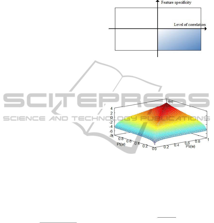
Figure 1: Feature selection. Based on the correlation with

the label, the features can be split into features weakly cor-

related with the label (left) and features highly correlated

with the label (right). Based on how speciﬁc the features

are, they can be split into domain speciﬁc features (top) and

generalizable features (bottom). Our goal is to select the

features in the bottom-right quadrant.

Figure 2: Ranking of features in the source domain using

Equation (1). The rank of a feature is higher if it has a high

probability or occurs with similar probability in the target

domain. Note: This graph was drawn using Octave (Eaton

et al., 2008).

value is the more inﬂuence the numerator has in rank-

ing the features, and vice versa. To limit its inﬂuence

on ranking the features, we chose a small value for

this parameter, 0.0001. The probability of a feature in

either domain is

P(w) =

N(w) + β

|D| + 2 ·β

(2)

where N is the number of instances in the domain in

which the feature w occurs, D is the total number of

instances in the domain and β is a smoothing factor,

which is used to prevent the probability of a feature

to be 0 (which would make the numerator in (1) equal

to 0, and the logarithm function is undeﬁned for 0).

We chose a small value for β as well, 0.0001, to limit

its inﬂuence on the ranking of features. Note that the

values for α and β do not have to be the same, but they

can be, as used by Tan et al. (2009) and in our case.

BIOINFORMATICS2013-InternationalConferenceonBioinformaticsModels,MethodsandAlgorithms

3.2 Multinomial Na

ıve Bayes (MNB)

Classiﬁer

The multinomial na

ıve Bayes classiﬁer (Mccallum

and Nigam, 1998) assumes that the sample data used

to train the classiﬁer is representative of the popula-

tion data on which the classiﬁer will be used. In ad-

dition, it assumes that the frequency of the features

determines the label assigned to an instance, and that

the position of a feature is irrelevant (the na

ıve Bayes

assumption). Thus, using Bayes’ property a classi-

ﬁer can approximate the posterior probability, i.e., the

probability of a class given an unclassiﬁed instance,

as being proportional to the product of the prior prob-

ability of the class, and the feature conditional proba-

bilities given an instance from the sample data:

P(c

| d

) ∝ P(c

)

∏

t∈|V |

[P(w

| c

)]

t,i

(3)

where the probability of the class is

P(c

) =

∑

i∈|D|

P(c

| d

)

|D|

(4)

and the conditional probability is

P(w

| c

) =

∑

i∈|D|

t,i

· P(c

| d

) + 1

∑

t∈|V |

∑

i∈|D|

t,i

· P(c

| d

) + |V |

(5)

Here, N

t,i

is the number of times feature w

occurs in

instance d

, |V | is the number of features, and |D| is

the number of instances.

3.3 Adapted Na

ıve Bayes Classiﬁer for

Biological Sequences

One limitation of the MNB classiﬁer is that it can only

be trained on one domain, and when the trained clas-

siﬁer is used on a different domain, in most cases, its

classiﬁcation accuracy decreases. To address this, we

used the Adapted Na

ıve Bayes (ANB) classiﬁer pro-

posed by Tan et al. (2009), with two modiﬁcations:

we used the labeled data from the target domain, and

employed the self-training technique. These will be

described in more detail shortly.

The ANB algorithm is a combination of the

expectation-maximization (EM) algorithm and a

weighted multinomial Na

ıve Bayes algorithm. Sim-

ilar to the EM algorithm, it has two steps that are

iterated until convergence. In the ﬁrst step, the M-

step, we simultaneously calculate the class probabil-

ity and the class conditional probability of a feature.

However, unlike the EM algorithm that uses the data

from one domain to calculate these values, this algo-

rithm uses a weighted combination of the data from

the source domain and the target domain.

P(c

) =

(1 − λ)

∑

i∈D

P(c

| d

) + λ

∑

i∈D

P(c

| d

)

(1 − λ)|D

| + λ|D

(6)

P(w

| c

) =

(1 − λ)(η

t,k

) + λN

t,k

+ 1

(1 − λ)

∑

t∈|V|

t,k

+ λ

∑

t∈|V|

t,k

+ 1

(7)

where N

t,k

is the number of times feature w

occurs in

a domain in instances labeled with class k:

t,k

∑

i∈D

t,i

P(c

| d

) (8)

λ is the weight factor between the source and target

domains:

λ = min{δ · τ, 1} (9)

and τ is the iteration number, δ ∈ (0, 1) is a constant

that determines how fast the weight shifts from the

source domain to the target domain, and η

is 1 if fea-

ture t in the source domain is a generalizable feature,

0 otherwise.

Unlike the algorithm proposed by Tan et al.

(2009), which considers that all the instances from

the target domain are unlabeled and does not use them

during the ﬁrst iteration (i.e., λ = 0), it is reasonable

to assume that there is a small number of labeled in-

stances in the target domain, and our algorithm uses

any labeled data from the target domain in the ﬁrst

and subsequent iterations. In the ﬁrst iteration we use

only labeled instances from the source and target do-

mains to calculate the probability distributions for the

class conditional probabilities given the instance. In

subsequent iterations we use the class of the instance

for the labeled data from the source and target do-

mains and the probability distribution of the class for

the unlabeled data from the target domain.

In the second step, the E-step, we estimate the

probability of the class for each instance with the val-

ues obtained from the M-step.

P(c

| d

) ∝ P(c

)

∏

t∈|V|

[P(w

| c

)]

t,i

(10)

The second modiﬁcation we made to the ANB

classiﬁer (Tan et al., 2009), is our use of self-training,

i.e., at each iteration, we select, proportional to the

class distribution, the instances with the top class

probability, and consider these to be labeled in the

subsequent iterations. This improves the prediction

accuracy of our classiﬁer because it does not allow

the unlabeled data to alter the class distribution from

the target labeled data.

NaïveBayesDomainAdaptationforBiologicalSequences

1 Load the data from the source domain, D

, the tar-

get domain, D

, and parameters α, β, δ.

2 Select generalizable features from the source do-

main, i.e., the top ranked features using Equation

(1).

3 For each class simultaneously calculate the class

probability and the class conditional probability

of each feature using Equations (6-7). For the

source domain use all labeled instances, and only

the generalizable features. For the target domain

use only labeled instances, and all features.

4 Select, proportional to the class distribution, the

target instances with the top class probability, and

consider these to be labeled in the subsequent it-

erations.

5 Loop until the labels assigned to unlabeled data

don’t change.

5.a M-step. Same as step 3 but use the class for la-

beled and self-trained instances from the target

domain, and the class distribution for unlabeled

instances.

5.b Same as step 4.

5.c E-step. Calculate the class distribution for un-

labeled training instances from the target do-

main using Equation (10).

6 Use classiﬁer to label new target data.

Figure 3: Outline of the Adapted Na

ıve Bayes algorithm for

biological sequences.

The two steps, E and M, are repeated until the

instance conditional probabilities values in (10) con-

verge (or a given number of iterations is reached). The

algorithm is summarized in Figure 3.

3.4 Data Sets

We used two data sets to evaluate our classiﬁer. The

ﬁrst data set, PSORTb v2.0

(Gardy et al., 2005),

was ﬁrst introduced in (Gardy et al., 2003), and con-

tains proteins from gram-negative and gram-positive

bacteria and their primary localization information:

cytoplasm, inner membrane, periplasm, outer mem-

brane, and extracellular space. For our experiments,

we identiﬁed classes that appear in both datasets, and

used 480 proteins from gram-positive bacteria (194

from cytoplasm, 103 from inner membrane, and 183

from extracellular space) and 777 proteins from gram-

Downloaded from http://www.psort.org/dataset/

datasetv2.html

negative bacteria (278 from cytoplasm, 309 from in-

ner membrane, and 190 from extracellular space).

The second data set, TargetP

, was ﬁrst introduced

in (Emanuelsson et al., 2000), and contains plant and

non-plant proteins and their subcellular localization:

mitochondrial, chloroplast, secretory pathway, and

“other.” From this data set we used 799 plant pro-

teins (368 mitochondrial, 269 secretory pathway and

162 “other”) and 2,738 non-plant proteins (371 mito-

chondrial, 715 secretory pathway and 1652 “other”).

Predicting protein localization is an important biolog-

ical problem because the function of the proteins is

related to their localization.

3.5 Data Preparation and Experimental

Setup

We represent each sequence as a count of occurrences

of k-mers. We use a sliding window approach to count

the k-mer frequencies. For example, the protein se-

quence LLRSYRS would be transformed when using

2-mers into 1, 1, 2, 1, 1 which are the counts corre-

sponding to the occurrences of features LL, LR, RS,

SY, YR.

In order to obtain unbiased estimates for classi-

ﬁer performance we used ﬁve-fold cross validation.

We use all labeled data from the source domain for

training (tSL) and randomly split the target domain

data into 3 sets: 20% used as labeled data for training

(tTL), 60% used as unlabeled data for training (tTU),

and 20% used as test data (TTL). So, we train our

classiﬁer on tSL + tTL + tTU and test it on TTL.

We wanted to answer several questions - speciﬁ-

cally, how does the performance of the classiﬁer vary

with:

Q1 Features used (i.e., 3-mers, 2-mers, or 1-mers)?

Q2 Number of features used in the target domain (i.e.,

keep all features, remove at most 50% of the least

occurring features)?

Q3 Number of features retained in the source domain

after selecting the generalizable features?

Q4 Variation with the size of the target la-

beled/unlabeled data set (i.e., train on 100% tSL

+ x% tTL + y% tTU, where x ∈ {5, 10, 20} and

y ∈ {20, 40, 60})?

Q5 The distance between the source and target do-

mains?

Q6 The choice of the source and target domains?

Downloaded from http://www.cbs.dtu.dk/services/

TargetP/datasets/datasets.php

BIOINFORMATICS2013-InternationalConferenceonBioinformaticsModels,MethodsandAlgorithms

As baselines, we compared our classiﬁer (ANB)

with the multinomial Na

ıve Bayes classiﬁer trained

on all source data (MNB s), the multinomial Na

ıve

Bayes classiﬁer trained on 5% target data (MNB 5t),

and the multinomial Na

ıve Bayes classiﬁer trained

on 80% target data (MNB 80t). Each classiﬁer was

tested on 20% of target data. The expectation is that

the prediction accuracy of our classiﬁer will be lower

bounded by MNB 5t, upper bounded by MNB 80t,

and be better than MNB s.

To evaluate our classiﬁer we used the area under

the receiver operating characteristic (auROC), as the

class distributions are relatively balanced.

3.6 Results

This section provides empirical evidence that aug-

menting the labeled data from a source domain with

labeled and unlabeled data from the target domain

with the ANB algorithm improves the classiﬁcation

accuracy compared to using only the limited labeled

data from the target domain or using only the data

from a source domain with the MNB classiﬁer.

Table 1 shows the average auROC values over the

ﬁve-fold cross validation trials for our algorithm and

for the baseline algorithms on the two datasets used.

For our algorithm, we used different amounts of la-

beled and unlabeled data from the target domain. For

example, the top-left value is the auROC for our algo-

rithm trained on 5% labeled data and 20% unlabeled

data. In each subtable the largest auROC value for the

ANB is highlighted.

We noted that the performance of the ANB classi-

ﬁer varies, as follows:

A1 The best results were obtained when using 3-mers

as features. This makes sense since longer k-mers

capture more information associated with the rel-

ative position of each amino-acid. When using

3-mers, our algorithm provides between 9.84%

and 34.14% better classiﬁcation accuracy when

compared to multinomial Na

ıve Bayes classiﬁer

trained on 5% of the labeled data from the tar-

get domain, and between 0.37% and 28.2% when

compared to the multinomial Na

ıve Bayes clas-

siﬁer trained on labeled data from the source do-

main, except when the plant proteins are the target

domain.

A2 When trying to establish how many features from

the target domain should be used we determined

that removing any features does not improve the

performance of our algorithm.

A3 When trying to ascertain how many features from

the source domain should be kept after ranking

them with Equation 1, we determined that the best

results were obtained when at least 50% of the

features were kept, i.e., the 50% top-ranked fea-

tures and any other features with the same rank as

the last feature kept.

A4 For most cases, the largest auROC values for

our algorithm were obtained when using the least

amount of target unlabeled data. This would sug-

gest that even though using unlabeled data is ben-

eﬁcial, using too much unlabeled data is detrimen-

tal because the unlabeled instances act as noise

and corrupt the prediction from the target labeled

data. In addition, intuitively, using more labeled

data from the target domain should lead to bet-

ter prediction accuracy. This was indeed the case

with our classiﬁer.

A5 When the source and target domains are close the

classiﬁer learned is better. For example, the au-

ROC is higher for the PSORTb datasets than for

the TargetP datasets. Therefore, the closer the tar-

get domain is to the source domain the better the

classiﬁer learned.

A6 For the PSORTb dataset, the ANB classiﬁer

had better prediction accuracy when the gram-

negative proteins were used as the source domain

than when the gram-positive proteins were used

as the source domain. Similarly, for the TargetP

dataset, we obtained better predictions when us-

ing non-plant proteins as the source domain than

when using plant proteins as the source domain.

This is because in both cases there were more

gram-negative instances and more non-plant in-

stances, respectively, than gram-positive instances

and plant instances, respectively.

It is interesting to note that in some instances the

multinomial Na

ıve Bayes classiﬁer trained on the

source domain performed better than our algorithm.

This occurred mainly when our algorithm used 5% or

10% of the target labeled data and when the features

were 1-mers or 2-mers. However, this is somewhat

expected, as using very little labeled data from the tar-

get domain does not provide a representative sample

for the population, and using short k-mers does not

capture the relative position of the amino-acids.

3.7 Preliminary Results on a Third

Dataset

We have also done a preliminary analysis on a third

data set

, ﬁrst introduced in (Schweikert et al., 2008).

Downloaded from ftp://ftp.tuebingen.mpg.de/fml/

cwidmer/

NaïveBayesDomainAdaptationforBiologicalSequences

Table 1: A comparison between the Adapted Na

ıve Bayes classiﬁer (ANB), the multinomial Na

ıve Bayes classiﬁer trained

on all source data (MNB s), the multinomial Na

ıve Bayes classiﬁer trained on 5% target data (MNB 5t), and the multinomial

ıve Bayes classiﬁer trained on 80% target data (MNB 80t). The results are reported as average auROC values over ﬁve-

fold cross validation trials. For the ANB classiﬁer, the row headings indicated how much target unlabeled data was used in

training the classiﬁer and the column headings indicate how much target labeled data was used. The best values for the ANB

are highlighted. Note that ANB is bounded by MNB 5t and MNB 80t, and that ANB predicts more accurately as the length

of k-mers increases.

PSORTb dataset TargetP dataset

Gram-positive as source and gram-negative as target Plant as source and non-plant as target

Features are 1-mers Features are 1-mers

ANB

MNB s MNB 5t MNB 80t

ANB

MNB s MNB 5t MNB 80t

tTU\tTL 5% 10% 20% tTU\tTL 5% 10% 20%

20% 0.9142 0.9170 0.9208

0.9274 0.9218 0.9352

20% 0.6526 0.6984 0.7398

0.7638 0.7990 0.812840% 0.9068 0.9082 0.9168 40% 0.6290 0.6624 0.6916

60% 0.8900 0.9020 0.9190 60% 0.6088 0.6452 0.7040

Features are 2-mers Features are 2-mers

ANB

MNB s MNB 5t MNB 80t

ANB

MNB s MNB 5t MNB 80t

tTU\tTL 5% 10% 20% tTU\tTL 5% 10% 20%

20% 0.9358 0.9366 0.9394

0.9330 0.9190 0.9424

20% 0.6578 0.7184 0.7938

0.7862 0.8260 0.839640% 0.9284 0.9268 0.9390 40% 0.6212 0.6702 0.6934

60% 0.9292 0.9358 0.9350 60% 0.6028 0.6308 0.6714

Features are 3-mers Features are 3-mers

ANB

MNB s MNB 5t MNB 80t

ANB

MNB s MNB 5t MNB 80t

tTU\tTL 5% 10% 20% tTU\tTL 5% 10% 20%

20% 0.9380 0.9380 0.9424

0.9194 0.8580 0.9552

20% 0.7582 0.8144 0.8566

0.6682 0.6386 0.883640% 0.9262 0.9278 0.9314 40% 0.7404 0.7972 0.8346

60% 0.9134 0.9240 0.9308 60% 0.7618 0.7636 0.7796

Gram-negative as source and gram-positive as target Non-plant as source and plant as target

Features are 1-mers Features are 1-mers

ANB

MNB s MNB 5t MNB 80t

ANB

MNB s MNB 5t MNB 80t

tTU\tTL 5% 10% 20% tTU\tTL 5% 10% 20%

20% 0.9278 0.9320 0.9346

0.9360 0.9142 0.9556

20% 0.7296 0.7190 0.7704

0.7618 0.7366 0.851440% 0.8978 0.9326 0.9118 40% 0.6922 0.7196 0.7696

60% 0.8912 0.8728 0.9302 60% 0.6716 0.7340 0.7548

Features are 2-mers Features are 2-mers

ANB

MNB s MNB 5t MNB 80t

ANB

MNB s MNB 5t MNB 80t

tTU\tTL 5% 10% 20% tTU\tTL 5% 10% 20%

20% 0.9090 0.9452 0.9466

0.9442 0.8852 0.9616

20% 0.7824 0.7810 0.7868

0.7836 0.7508 0.885240% 0.9180 0.9206 0.9502 40% 0.7272 0.7514 0.7862

60% 0.9426 0.9428 0.9428 60% 0.7380 0.7362 0.7592

Features are 3-mers Features are 3-mers

ANB

MNB s MNB 5t MNB 80t

ANB

MNB s MNB 5t MNB 80t

tTU\tTL 5% 10% 20% tTU\tTL 5% 10% 20%

20% 0.9590 0.9520 0.9614

0.9578 0.8118 0.9544

20% 0.8200 0.8092 0.8596

0.8968 0.6860 0.862840% 0.9280 0.9440 0.9460 40% 0.7382 0.7442 0.7990

60% 0.9278 0.9282 0.9460 60% 0.6904 0.7256 0.7848

This dataset contains DNA sequences of 141 base

pairs centered around the donor splice site dimer AG

and the label of whether or not that AG dimer is a

true splice site. The sequences are from ﬁve organ-

isms, C.elegans as the source domain, and C.remanei,

P.paciﬁcus, D.melanogaster, and A.thaliana as target

domains. We used the dataset with 100,000 instances

for the source domain, and the datasets with 2,500,

6,500, 16,000, and 40,000 instances for the target do-

main. In each dataset there are about 1% positive

instances. Accurately predicting splice sites is im-

portant for genome annotation (R

atsch et al., 2007;

Bernal et al., 2007).

For this dataset we used the area under precision-

recall curve (auPRC), a metric that is preferred over

area under a receiver operating characteristic curve

BIOINFORMATICS2013-InternationalConferenceonBioinformaticsModels,MethodsandAlgorithms

when the class distribution is skewed, which is the

case with this dataset.

The results for this dataset were very poor, with

our algorithm always gravitating towards classifying

each instance as not containing a splice site. We be-

lieve that this is due mainly because the k-mers indi-

cating a splice site occur with low frequency and their

relative position to the splice site is important. We

will discuss in Section 4 how we propose to address

this issue in future work.

4 CONCLUSIONS AND FUTURE

WORK

In this paper, we proposed a domain adaptation classi-

ﬁer for biological sequences. This algorithm showed

promising classiﬁcation performance in our experi-

ments. Our analysis indicates that the closer the tar-

get domain is to the source domain the better is the

classiﬁer learned. Other conclusions drawn from our

observations: using 2-mers or 3-mers results in bet-

ter prediction, with small differences between them;

removing features from the target domain reduces the

accuracy of classiﬁer; having more target labeled data

increases the accuracy of classiﬁer; and adding too

much target unlabeled data decreases the accuracy of

classiﬁer.

In future work we would like to investigate how

would assigning different weights to the data used for

training inﬂuence the accuracy prediction of the algo-

rithm. We would like to assign higher weight to the

labeled data from the target domain since this is more

likely to correctly predict the class of the target test

data than the labeled data from the source domain or

the unlabeled data from the target domain.

We would also like to evaluate other methods for

selecting the generalizable features. For example,

we would like to investigate if selecting generalizable

features using the mutual information of the features

instead of their probabilities, in Equation (1), leads to

better classiﬁcation accuracy.

Another aspect we would like to improve is the

accuracy of this classiﬁer on the splice site dataset, to

get accuracy that is similar to state of the art splice

site classiﬁers, e.g., SVM classiﬁers. We would like

to reduce the number of motifs with different cluster-

ing strategies, and identify more discriminative mo-

tifs using Gibbs sampling or MEME. In addition, we

would like to run experiments on smaller splice site

datasets to better understand the characteristics of this

problem.

ACKNOWLEDGEMENTS

The computing for this project was performed on the

Beocat Research Cluster at Kansas State University,

which is funded in part by NSF grants CNS-1006860,

EPS-1006860, EPS-0919443, and MRI-1126709.

REFERENCES

Baten, A., Chang, B., Halgamuge, S., and Li, J. (2006).

Splice site identiﬁcation using probabilistic param-

eters and svm classiﬁcation. BMC Bioinformatics,

7(Suppl 5):S15.

Bernal, A., Crammer, K., Hatzigeorgiou, A., and Pereira,

F. (2007). Global discriminative learning for higher-

accuracy computational gene prediction. PLoS Com-

put Biol, 3(3):e54.

Brown, M. P. S., Grundy, W. N., Lin, D., Cristianini, N.,

Sugnet, C., Furey, T. S., M.Ares, J., and Haussler, D.

(2000). Knowledge-based analysis of microarray gene

expression data using support vector machines. PNAS,

97(1):262–267.

Dai, W., Xue, G., Yang, Q., and Yu, Y. (2007). Transferring

ıve bayes classiﬁers for text classiﬁcation. In Pro-

ceedings of the 22nd AAAI Conference on Artiﬁcial

Intelligence.

Degroeve, S., Saeys, Y., De Baets, B., Rouz

e, P., and Van

De Peer, Y. (2005). Splicemachine: predicting splice

sites from high-dimensional local context representa-

tions. Bioinformatics, 21(8):1332–1338.

Eaton, J. W., Bateman, D., and Hauberg, S. (2008). GNU

Octave Manual Version 3. Network Theory Ltd.

Emanuelsson, O., Nielsen, H., Brunak, S., and von Heijne,

G. (2000). Predicting subcellular localization of pro-

teins based on their N-terminal amino acid sequence.

Journal of molecular biology, 300(4):1005–1016.

Gardy, J. L., Laird, M. R., Chen, F., Rey, S., Walsh, C. J.,

Ester, M., and Brinkman, F. S. L. (2005). Psortb

v.2.0: Expanded prediction of bacterial protein sub-

cellular localization and insights gained from compar-

ative proteome analysis. Bioinformatics, 21(5):617–

623.

Gardy, J. L., Spencer, C., Wang, K., Ester, M., Tusn

ady,

G. E., Simon, I., Hua, S., deFays, K., Lambert, C.,

Nakai, K., and Brinkman, F. S. (2003). Psort-b:

improving protein subcellular localization prediction

for gram-negative bacteria. Nucleic Acids Research,

31(13):3613–3617.

Huang, J., Li, T., Chen, K., and Wu, J. (2006). An approach

of encoding for prediction of splice sites using svm.

Biochimie, 88:923–9.

Jaakkola, T. S. and Haussler, D. (1999). Exploiting gen-

erative models in discriminative classiﬁers. In Pro-

ceedings of the 1998 conference on Advances in neu-

ral information processing systems II, pages 487–493,

Cambridge, MA, USA. MIT Press.

Jiang, J. and Zhai, C. (2007). A two-stage approach to do-

main adaptation for statistical classiﬁers. In Proceed-

ings of the sixteenth ACM conference on Conference

NaïveBayesDomainAdaptationforBiologicalSequences

on information and knowledge management, CIKM

’07, pages 401–410, New York, NY, USA. ACM.

Lorena, A. C. and de Carvalho, A. C. P. L. F. (2003).

Human splice site identiﬁcation with multiclass sup-

port vector machines and bagging. In Proceedings of

the 2003 joint international conference on Artiﬁcial

neural networks and neural information processing,

ICANN/ICONIP’03, pages 234–241, Berlin, Heidel-

berg. Springer-Verlag.

Maeireizo, B., Litman, D., and Hwa, R. (2004). Co-training

for predicting emotions with spoken dialogue data. In

Proceedings of the ACL 2004 on Interactive poster

and demonstration sessions, ACLdemo ’04, Strouds-

burg, PA, USA. Association for Computational Lin-

guistics.

Mccallum, A. and Nigam, K. (1998). A comparison of event

models for naive bayes text classiﬁcation. In AAAI-98

Workshop on ’Learning for Text Categorization’.

uller, K.-R., Mika, S., R

atsch, G., Tsuda, S., and

Sch

olkopf, B. (2001). An introduction to kernel-based

learning algorithms. IEEE Transactions on Neural

Networks, 12(2):181–202.

Nigam, K., Mccallum, A., Thrun, S., and Mitchell, T.

(1999). Text classiﬁcation from labeled and unlabeled

documents using EM. In Machine Learning, pages

103–134.

Noble, W. S. (2006). What is a support vector machine?

Nat Biotech, 24(12):1565–1567.

Pan, S. J. and Yang, Q. (2010). A survey on transfer learn-

ing. IEEE Transactions on Knowledge and Data En-

gineering, 22(10):1345–1359.

atsch, G. and Sonnenburg, S. (2004). Accurate splice site

detection for caenorhabditis elegans. In B. Schlkopf,

K. T. and Vert, J.-P., editors, Kernel Methods in Com-

putational Biology, pages 277–298. MIT Press.

atsch, G., Sonnenburg, S., Srinivasan, J., Witte, H.,

uller, K.-R., Sommer, R., and Sch

olkopf, B. (2007).

Improving the c. elegans genome annotation using

machine learning. PLoS Computational Biology,

3:e20.

Riloff, E., Wiebe, J., and Wilson, T. (2003). Learning sub-

jective nouns using extraction pattern bootstrapping.

In Proceedings of the seventh conference on Natural

language learning at HLT-NAACL 2003 - Volume 4,

CONLL ’03, pages 25–32, Stroudsburg, PA, USA.

Association for Computational Linguistics.

Sch

olkopf, B. and Smola, A. J. (2001). Learning with Ker-

nels: Support Vector Machines, Regularization, Opti-

mization, and Beyond. MIT Press, Cambridge, MA,

USA.

Schweikert, G., Widmer, C., Sch

olkopf, B., and R

atsch,

G. (2008). An empirical analysis of domain adap-

tation algorithms for genomic sequence analysis. In

NIPS’08, pages 1433–1440.

Sonnenburg, S., R

atsch, G., Jagota, A., and M

uller, K.-R.

(2002). New methods for splice-site recognition. In

In Proceedings of the International Conference on Ar-

tiﬁcal Neural Networks., pages 329–336. Copyright

by Springer.

Sonnenburg, S., Schweikert, G., Philips, P., Behr, J., and

atsch, G. (2007). Accurate splice site prediction us-

ing support vector machines. BMC Bioinformatics,

8(Supplement 10):1–16.

Tan, S., Cheng, X., Wang, Y., and Xu, H. (2009). Adapting

naive bayes to domain adaptation for sentiment anal-

ysis. In Proceedings of the 31th European Confer-

ence on IR Research on Advances in Information Re-

trieval, ECIR ’09, pages 337–349, Berlin, Heidelberg.

Springer-Verlag.

Tsuda, K., Kawanabe, M., R

atsch, G., Sonnenburg, S.,

and M

uller, K.-R. (2002). A new discriminative

kernel from probabilistic models. Neural Comput.,

14(10):2397–2414.

Vapnik, V. N. (1995). The nature of statistical learning the-

ory. Springer-Verlag New York, Inc., New York, NY,

USA.

Yarowsky, D. (1995). Unsupervised word sense disam-

biguation rivaling supervised methods. In Proceed-

ings of the 33rd annual meeting on Association for

Computational Linguistics, ACL ’95, pages 189–196,

Stroudsburg, PA, USA. Association for Computa-

tional Linguistics.

Zhang, Y., Chu, C.-H., Chen, Y., Zha, H., and Ji, X. (2006).

Splice site prediction using support vector machines

with a bayes kernel. Expert Syst. Appl., 30(1):73–81.

Zien, A., R

atsch, G., Mika, S., Sch

olkopf, B., Lengauer, T.,

and M

uller, K.-R. (2000). Engineering support vec-

tor machine kernels that recognize translation initia-

tion sites. Bioinformatics, 16(9):799–807.

BIOINFORMATICS2013-InternationalConferenceonBioinformaticsModels,MethodsandAlgorithms