
Exploratory EEG Analysis using Clustering and Phase-locking Factor
Carlos Carreiras, Helena Aidos, Hugo Silva and Ana Fred
Instituto de Telecomunicac¸˜oes, Instituto Superior T´ecnico, Lisbon, Portugal
Keywords:
Emotions, EEG, ICA, EMD, Phase-locking Factor, Clustering.
Abstract:
Emotion recognition is essential for psychological and psychiatric applications and for improving the quality
of human-machine interaction. Therefore, a simple and reliable method is needed to automatically assess the
emotional state of a subject. This paper presents an application of clustering algorithms to feature spaces
obtained from the acquired EEG of subjects performing a stress-inducing task. These features were obtained
in three ways: using the EEG directly, using ICA to remove eye movement artifacts, and using EMD to extract
data-driven modes present in the signals. From these features, we computed band-power features (BPFs) as
well as pairwise phase-locking factors (PLFs), in a total of six different feature spaces. These six feature
spaces are used as input to various clustering algorithms. The results of these clustering techniques show
interesting phenomena, including prevalence for low numbers of clusters and the fact that clusters tend to be
made of consecutive test lines.
1 INTRODUCTION
Emotions play a pivotal role in human communica-
tion, sometimes even more important than the actual
ideas being transmitted. For instance, imagine your-
self vacationing in a foreign country, not understand-
ing the local language. Naturally, there is a gaping
language barrier in any communication attempt. Nev-
ertheless, you can easily and intuitively gage the emo-
tional state of your interlocutor, knowing if s/he is be-
ing aggressive, pleasant, sad, happy, etc., allowing to
infer, in rough terms, what is going on. Indeed, the
need to communicate emotion has inspired the devel-
opment of the famous emoticons for text-based Inter-
net chatting, though the participants may not always
be truthful (Herbert, 2012).
However, this aspect of communication is lacking
in human-machine interaction, where the machines
(e.g. your personal computer) cannot understand nor
produce emotional cues, which could potentially aug-
ment the interaction quality. Therefore, there is a need
to, by simple and reliable means, assess the emo-
tional state of a person, not only in the context of
human-machine interaction, but also in psychologi-
cal and psychiatric studies, which many times rely
on self-evaluation questionnaires to assess the emo-
tions elicited during the experiments (Coan and Allen,
2007).
One possible approach to automatic emotion reco-
gnition is by analyzing the subject’s biosignals (e.g.
electrodermal activity, blood-volume-pulse, periph-
eral temperature, electrocardiogram signals) during
emotion elicitation (Canento et al., 2011). In partic-
ular, the electroencephalogram (EEG) is a noninva-
sive, cost effective and simple technique, with good
temporal resolution (Mak and Wolpaw, 2009), pro-
viding a measure of what is happening in the brain,
the physiological source of emotions. It has long been
noted that the EEG can provide information about the
emotional state of the subject, in particular regard-
ing frontal asymmetries (Ahern and Schwartz, 1985;
Coan and Allen, 2004). In this paper, we make an ex-
ploratory analysis of the EEG acquired from subjects
performing a stressful task, demanding high concen-
tration levels over a long period of time. This exper-
iment mimics what may happen during an interactive
educational game, where it would be useful to de-
tect when the subject is growing tired of performing a
certain task, seamlessly switching to another, less de-
manding activity.
Traditionally, EEG signals are analyzed by ex-
tracting band power features, given that brain ac-
tivity, as measured from the scalp, exhibits an os-
cillatory behavior whose dynamics (amplitude, fre-
quency and phase) are modulated by the various neu-
rological tasks (Pfurtscheller and Lopes da Silva,
1999). For example, the task of movement prepa-
ration induces a decrease of the EEG power in the
79
Carreiras C., Aidos H., Silva H. and Fred A..
Exploratory EEG Analysis using Clustering and Phase-locking Factor.
DOI: 10.5220/0004251300790088
In Proceedings of the International Conference on Bio-inspired Systems and Signal Processing (BIOSIGNALS-2013), pages 79-88
ISBN: 978-989-8565-36-5
Copyright
c
2013 SCITEPRESS (Science and Technology Publications, Lda.)

motor cortex, termed Event-Related Desynchroniza-
tion (Pfurtscheller and Lopes da Silva, 1999). How-
ever, band power features require the selection of the
frequency bands, which may change from subject to
subject. An alternative method to analyze the EEG,
the Phase-Locking Factor (PLF), has been proposed
in the field of Brain-Computer Interfaces (Carreiras
et al., 2012), which we apply here in the context of
emotion analysis. This measure may be useful in the
sense that, as a synchronization measure, it can iden-
tify the previously mentioned frontal asymmetries ob-
served in the EEG.
This paper is organized as follows: Section 2 de-
scribes the process used to obtain the EEG signals.
Section 3 details the methodology proposed in this
paper,which consists of three main stages: signal pro-
cessing (section 3.1), feature extraction (section 3.2)
and clustering (section 3.3). Section 4 presents the re-
sults obtained after applying this methodology to the
EEG data. Section 5 and section 6 discuss these find-
ings and present concluding remarks, respectively.
2 EMOTION ELICITATION AND
DATA ACQUISITION
The EEG signals were obtained in the context of
the HiMotion project (Gamboa et al., 2007), an ex-
periment to acquire information related to human-
computer interaction and physiological signals on dif-
ferent cognitive activities. The signals were acquired
at four scalp locations according to the 10-20 system
(F
p1
, F
z
, F
p2
, and O
z
– see Figure 1), with a sampling
frequency of 256 Hz.
Figure 1: Location of the acquired electrodes (red).
During the acquisition, the subjects were asked to
perform various interactive cognitive tasks. In partic-
ular, a concentration task was performed, inspired in a
test from the MENSA set (Fulton, 2000). In this test,
the subject is given a matrix (20 lines by 40 columns)
of integers. The goal is to identify, line by line, pairs
of consecutive numbers that add to 10 (see Figure 2).
This task is cognitively demanding, as the pairs can
be consecutive (i.e. the same number can be used in
more than one pair), and therefore the test measures
the capability of the subject to maintain concentra-
tion over a long period of time, being expected to be
stress-inducing. EEG data was recorded from 24 sub-
jects (17 males and 7 females) with ages in the range
23.3±2.4 years.
Figure 2: Example matrix of the concentration test; the user
selects, line by line, the pairs of consecutive numbers that
add to 10.
3 THE PROPOSED
METHODOLOGY
In order to analyze the EEG signals obtained as de-
scribed in section 2, we propose the methodologypre-
sented in figure 3. This methodology starts with a fil-
tering stage, following by a denoising process using
independent component analysis (ICA) and empiri-
cal mode decomposition (EMD). The EEG features
are obtained in the feature extraction stage using two
different measures: band-power features (BPF) and
phase-locking factor (PLF). Finally, several cluster-
ing algorithms are applied to each of the six feature
spaces and the results are analyzed to detect changes
in the emotional state. All these stages are explained
in detail in the following subsections.
3.1 Signal Processing
In order to eliminate noise from non-biological
sources (power-line noise, baseline wander, etc.), the
raw EEG was processed with two Butterworth filters,
applied with both a forward and a backward pass, to
avoid phase disruptions: one high-pass filter, order 8,
with cutoff frequency at 4 Hz and one low-pass fil-
ter, order 16, with cutoff frequency at 40 Hz. How-
BIOSIGNALS2013-InternationalConferenceonBio-inspiredSystemsandSignalProcessing
80
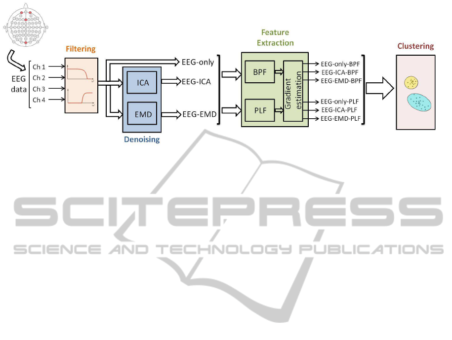
Figure 3: Scheme with the proposed methodology.
ever, the resulting signal is still fraught with biologi-
cal artifacts, such as eye blinks, eye movements, and
other muscle contractions. Therefore, three distinct
paths were evaluated to later apply the feature extrac-
tion algorithms. The first, and simplest approach ap-
plies no further noise reduction, which we will call as
the EEG-only approach, based on the filtered EEG.
The second approach uses Independent Component
Analysis (ICA) in an attempt to reduce the impact
of eye artifacts (denoted as EEG-ICA). Finally, the
last solution employs Empirical Mode Decomposition
(EMD), a method to analyze nonstationary and non-
linear data (denoted as EEG-EMD).
3.1.1 Independent Component Analysis
In the blind source separation problem (BSS), let X =
[X
1
, ..., X
M
]
T
(M being the number of signals) be the
observed data produced by a linear mixture of some
source signals S = [S
1
, ..., S
N
]
T
(N being the number
of sources), defined by the M ×N matrix A:
X = AS. (1)
The crux of the BSS problem is how to estimate
the sources S and the mixing matrix A from the ob-
served signals X. One of the available methods to do
so is Independent Component Analysis (ICA). The
ICA method estimates the sources by optimizing a
measure of their independence, resulting in sources
that are maximally independent (Hyv¨arinen et al.,
2001).
It has been shown that the ICA method is effec-
tive at separating neural activity from muscle and
blink artifacts in EEG data (Jung et al., 2000). In
this paper, we use the ubiquitous FastICA algorithm
(Hyv¨arinen, 1999) to decomposethe filtered EEG into
its independent components, although other alterna-
tives are available in the literature, such as the EFICA
(Koldovsky et al., 2006) or Extended Infomax (Lee
et al., 2006) algorithms. We then visually identi-
fied and eliminated the component that best isolated
the eye artifacts, reconstructing the EEG without that
component. Note that, as the acquired EEG signals
only have four channels, we chose to remove just
one of the components. An example of the original
EEG signal, its ICA decomposition and reconstruc-
tion without the noisy component can be seen in Fig-
ure 4.
3.1.2 Empirical Mode Decomposition
The Empirical Mode Decomposition algorithm de-
composes a given signal into a series of Intrin-
sic Mode Function (IMFs), using a sifting process
(Huang et al., 1998). This data-driven method pro-
duces components whose number of extrema differs
from the number of zero crossings, at most, by one,
and, additionally, at any point, the local mean is zero
(in an envelope defined by the local maxima and min-
ima). The sum of the IMFs approximates the original
signal, thus guaranteeingcompleteness of the method.
Each IMF is associated with the intrinsic time scales
of the signal, from fine temporal scales (high fre-
quency modes) to coarse temporal scales (low fre-
quency modes).
In this paper, each EEG signal was decomposed
with the EMD method, selecting the IMFs with mean
energy above 5% of the maximum energy. The result-
ing components were treated as EEG-like signals for
the subsequent processing steps.
3.2 Feature Extraction
The EEG features extracted in this paper arise from
two different approaches to evaluate mental activity.
The first approach uses the traditional band power fea-
tures (BPF), by computing the average power in a se-
ries of appropriate frequency bands (Section 3.2.1).
ExploratoryEEGAnalysisusingClusteringandPhase-lockingFactor
81
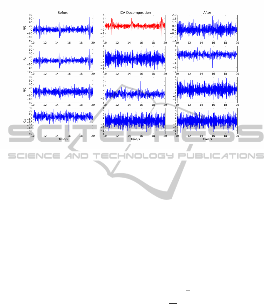
Figure 4: Example of applying the ICA method to remove eye artifacts from the EEG; the left column shows the four
original EEG channels, where the spikes are the eye artifacts; the middle column shows the ICA decomposition, with removed
component in red; and the right column presents the reconstructed EEG.
The second approach uses a method of synchroniza-
tion quantification, the Phase-Locking Factor (PLF –
Section 3.2.2). However, one of the difficulties of an-
alyzing the biosignals resulting from a continuously
interactive experiment, such as presented here, is the
fact that different subjects will conclude the task in
different time intervals. In this particular case, there
is variability in the time a subject takes to conclude
each line of the Concentration test, and, consequently,
in the total length of the task. Therefore, a method
based on a Gradient Estimation was used to evaluate
the trend of both types of features (BPF and PLF) over
time, obtaining a value for each line of the concentra-
tion test (Section 3.2.3).
Note that each of the preprocessing alternatives
(EEG-only, EEG-ICA and EEG-EMD) was analyzed
with both kinds of feature extraction (BPF and PLF),
resulting in 6 different sets of features. For clarity, we
denote each set by the combination of the preprocess-
ing name and the feature extraction method. For in-
stance, the feature set “EEG-ICA-PLF” was obtained
by extracting the PLF features from the EEG prepro-
cessed by the ICA method.
3.2.1 Band Power Features
For the Band Power Features, the following bands
were considered:
• Theta Band: from 4 Hz to 8 Hz;
• Lower Alpha Band: from 8 Hz to 10 Hz;
• Upper Alpha Band: from 10 Hz to 13 Hz;
• Beta Band: from 13 Hz to 25 Hz;
• Gamma Band: from 25 Hz to 40 Hz.
The features were extracted, for each channel, by
computing a short-time Fourier transform in windows
of 500 ms, with 50% overlap, padding the windowed
signal with zeros up to 1024 samples. An order 5
median filter was then applied to the resulting time-
courses.
3.2.2 Phase-locking Factor
Given two oscillators with phases φ
i
[n] and φ
k
[n], n =
1, ..., T (with T the number of discrete time samples),
the PLF is defined as (Almeida et al., 2011):
ρ
ik
=
1
T
T
∑
n=1
e
j(φ
i
[n]−φ
k
[n])
, (2)
where j =
√
−1 is the imaginary unit. This measure
ranges from 0 to 1. While the value ρ
ik
= 1 corre-
sponds to perfect synchronization between the two
signals (constant phase lag), the value ρ
ik
= 0 cor-
responds to no synchronization. Put simply, the PLF
assesses whether the difference between the phases
of the oscillators are strongly or weakly clustered
around some angle in the complex unitary circle. In
this work, the phase information is extracted from the
EEG signals through the concept of analytical signals,
which is done by applying the Hilbert transform to the
BIOSIGNALS2013-InternationalConferenceonBio-inspiredSystemsandSignalProcessing
82

signal. Given a real signal x(t), its Hilbert transform
is defined as H
t
{x} = x(t) ∗
1
πt
, where ∗ denotes the
convolution operator; then, the corresponding analyt-
ical signal z(t) is obtained as:
z(t) = x(t) + jH
t
{x} = x(t) + j
x(t) ∗
1
πt
. (3)
The PLF was computed, for all possible electrode
pairs, in windows of 250 ms, with 50% overlap. An
order 5 median filter was then applied.
3.2.3 Gradient Estimation
In order to estimate the trend, over time, of the feature
sets, a straight line was fitted to each line k = 1, ..., 20
of the concentration task (with T(k) duration), esti-
mating the gradient G(k) of that line. The evolution
of the features, from the initial state, over the lines is
then given by D(k):
D(k) = D(k −1) + G(k) ×T(k) (4)
with D(0) = 0. With this methodology we obtain,
for each line of the concentration task, a feature vec-
tor that characterizes that line. The dimension of the
feature vector depends both on the type of denois-
ing (EEG-only, ICA, EMD) and the feature extrac-
tion method (BPF, PLF). Denoting as C the number
of channels at the output of the denoising step, the
BPF method produces 5 ×C features per line (5 fre-
quency bands), while the PLF method produces
C
2
features (combinations of C choose 2, without repeti-
tions). The feature sets are then fed to the clustering
algorithms described in the following subsection.
3.3 Clustering Algorithms
Clustering consists in grouping objects that share
some characteristics. To identify which objects
should be grouped together, we need some similar-
ity measure such as the Euclidean distance. Cluster-
ing algorithms can be divided in two major categories:
hierarchical and partitional algorithms.
Hierarchical clustering algorithms output a tree
structure of nested objects, called dendrogram; one
can cut the dendrogram to obtain a partition of the
data. The level to cut the dendrogram can be de-
cided based on the lifetime of the clusters (Theodor-
idis and Koutroumbas, 2009); we use the largest life-
time criterion (Fred and Jain, 2002) in all of our ex-
periments. Examples of typical hierarchical algo-
rithms are single-link, average-link and ward-linkage
(Theodoridis and Koutroumbas, 2009).
Partitional clustering algorithms simply assign an
object to a single cluster. The simplest and most
widespread algorithm in this category is k-means
(Jain, 2010).
In this paper, we will apply various clustering
algorithms to the six feature spaces defined in sec-
tion 3.2 (EEG-only-BPF, EEG-ICA-BPF, etc). We
apply average-link (AL) and ward-linkage (WL) to
those datasets; these two algorithmsdiffer in how they
measure the distance between two clusters. The AL
algorithm uses the average distance for all pairs of
points, one in one cluster and one in the other. It is
an algorithm that tends to merge clusters with small
variances and takes into account the cluster structure.
The WL algorithm is based on the increase in sum of
squares within clusters, after merging, summed over
all points. This algorithm tends to find same-size,
spherical clusters and it is sensitive to outliers.
Recently, a single-link based algorithm has been
proposed using a dissimilarity measure based on
triplets of points, called dissimilarity increments, in-
stead of pairwise dissimilarities (Aidos and Fred,
2011). This algorithm uses the same principle for the
choice of clusters to merge as single-link; however,
the decision of merging two clusters or not is based
on the distribution of the dissimilarity increments. In
this paper, we will use average-link and ward-linkage
based algorithms following the same principle of dis-
similarity increments; we will call them ALDID and
WLDID.
Finally, we will also apply k-means to the signals,
with k set to 2 and 3.
4 EXPERIMENTAL RESULTS
4.1 Band Power Features
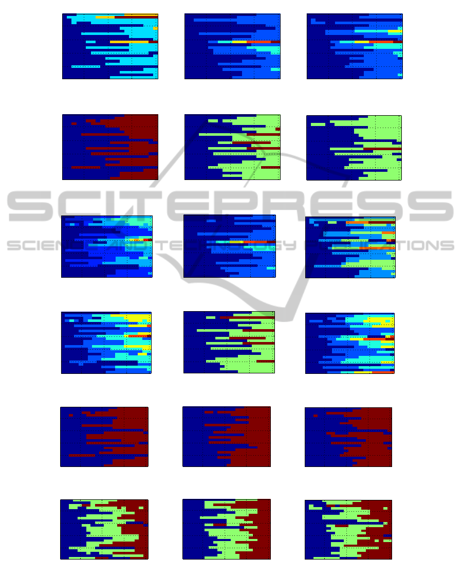
Figure 5 shows the results using the three BPF feature
spaces; different clusters are denoted using different
colors. There are a few major conclusions across all
subjects and clustering algorithms. In the vast major-
ity of cases, the lifetime criterion selects a lownumber
of clusters; usually 2 and sometimes 3, with 4 or more
clusters being very rare. Furthermore, again in the
majority of cases, each cluster consists of intervals of
test lines. For example, subject 24, when analyzed us-
ing EEG-only-BPF and AL (top-left subfigure in fig-
ure 5), has the first 10 test lines in one cluster and the
last 10 test lines in the other cluster. There are few
exceptions to this, such as subject 4 on the same sub-
figure (which has one cluster consisting of test lines 1,
2, 4, 5 and 6, which is not an interval because it does
not contain test line 3).
Since clusters usually correspond to intervals of
test lines, in the majority of cases it makes sense to
ExploratoryEEGAnalysisusingClusteringandPhase-lockingFactor
83
test line
subjects
EEG−only−BPF −− AL
5 10 15 20
5
10
15
20
test line
subjects
EEG−ICA−BPF −− AL
5 10 15 20
5
10
15
20
test line
subjects
EEG−EMD−BPF −− AL
5 10 15 20
5
10
15
20
test line
subjects
EEG−only−BPF −− WL
5 10 15 20
5
10
15
20
test line
subjects
EEG−ICA−BPF −− WL
5 10 15 20
5
10
15
20
test line
subjects
EEG−EMD−BPF −− WL
5 10 15 20
5
10
15
20
test line
subjects
EEG−only−BPF −− ALDID
5 10 15 20
5
10
15
20
test line
subjects
EEG−ICA−BPF −− ALDID
5 10 15 20
5
10
15
20
test line
subjects
EEG−EMD−BPF −− ALDID
5 10 15 20
5
10
15
20
test line
subjects
EEG−only−BPF −− WLDID
5 10 15 20
5
10
15
20
test line
subjects
EEG−ICA−BPF −− WLDID
5 10 15 20
5
10
15
20
test line
subjects
EEG−EMD−BPF −− WLDID
5 10 15 20
5
10
15
20
test line
subjects
EEG−only−BPF −− 2−means
5 10 15 20
5
10
15
20
test line
subjects
EEG−ICA−BPF −− 2−means
5 10 15 20
5
10
15
20
test line
subjects
EEG−EMD−BPF −− 2−means
5 10 15 20
5
10
15
20
test line
subjects
EEG−only−BPF −− 3−means
5 10 15 20
5
10
15
20
test line
subjects
EEG−ICA−BPF −− 3−means
5 10 15 20
5
10
15
20
test line
subjects
EEG−EMD−BPF −− 3−means
5 10 15 20
5
10
15
20
Figure 5: Clustering results for the EEG-BPF data. Each column corresponds to one type of data processing (from left
to right: EEG-only, ICA, EMD) and each row corresponds to one clustering algorithm (from top to bottom: average-link,
ward-linkage, ALDID, WLDID, 2-means and 3-means). In each subfigure, the horizontal axis spans the 20 test lines, and the
vertical axis spans the 24 subjects. Each different color denotes a different cluster.
BIOSIGNALS2013-InternationalConferenceonBio-inspiredSystemsandSignalProcessing
84

define transition test lines, which are the first test line
of each interval of test lines in the same cluster, except
the initial test line. For example, for subject 24 using
EEG-only-BPF and AL, test line 11 is a transition test
line. A third global conclusion is that the transition
test lines tend to occur in the middle of the horizontal
axis, and less on the edges. The exceptions to this are
(EEG-only-BPF and ALDID), (EEG-only-BPF and
WLDID), (EEG-EMD-BPF and ALDID) and (EEG-
EMD-BPF and WLDID).
These transition test lines may correspond to sev-
eral things; for example, it might indicate a test line
where the subject began to feel more comfortablewith
the task, or it might indicate a time where the subject
began growing tired of maintaining high concentra-
tion levels. Further work, where subjects are queried
about their emotional state during the experiments, or
where test lines of different difficulties are used as a
proxy of stress level, is required to corroborate this
claim.
Still regarding figure 5, there are a few other in-
teresting conclusions. Subject 11 appears to be some-
what of an outlier: usually, all other subjects have 2-3
clusters, whereas subject 11 has many more (for ex-
ample, he/she has 6 on EEG-ICA-BPF using AL or
ALDID). This might suggest that something different
happened for this subject, such as improper experi-
mental setup or inability to understand the given in-
structions.
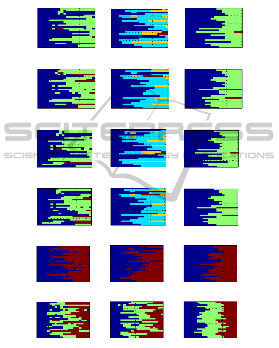
4.2 Phase-locking Factor
Figure 6 conveys the same information as figure 5,
but using the PLF features instead of the BPF ones.
Again, the majority of subjects yield clusters which
are composed of consecutivetime intervals. However,
and unlike figure 5, the number of clusters (and transi-
tions) is much smaller using the PLF features than us-
ing the BPF ones: the ICA features have a maximum
of 4 clusters on some subjects, and the EEG-only and
EMD ones have a maximum of 3.
There is a striking aspect in the EMD figures
(rightmost column): all cases have clusters made of
an interval, with no exceptions. Furthermore, in these
cases, there is never any transition in the first 4 test
lines, nor on the last 2, and in the vast majority of
cases the transitions occur in the central part of the
figures (test lines 7 to 13 or so). This is markedly
different from the EEG-only cases (leftmost column)
where some subjects have non-interval clusters and
where transitions occur throughout the 20 test lines.
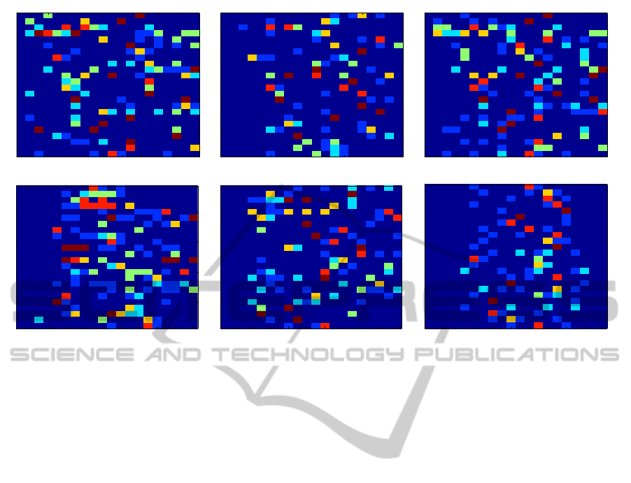
5 DISCUSSION
To further study the centrality of the transitions in the
EEG-EMD-PLF results, we computed the number of
algorithms which have a transition in test line t, for
each subject and each feature space. This is shown
in figure 7, where the horizontal and vertical axes are
similar to the previous figures, but now the color in-
dicates the number of algorithms where a transition
occurred in that test line for that subject. The values
range from 0 (no algorithms) to 6 (all algorithms). In
these plots, the centrality of the transitions for EEG-
EMD-PLF is clearly visible; it is also clear that the
other five feature spaces do not have this behavior.
This is an interesting find which we plan to actively
investigate in the future, which may or may not be
related to the subject’s emotional state.
Another interesting find for the EEG-EMD-PLF
case is that the vast majority of cases are either very
few transitions (0 or 1) or many transitions (5 or 6),
with few cases of intermediate numbers of transitions.
This indicates that the various clustering algorithms
agree with each other a lot more for the EEG-EMD-
PLF case than for all other cases. This agreement sug-
gests that some underlying (possibly emotional) phe-
nomenon is being captured by the use of EMD and
PLF which is missed otherwise.
6 CONCLUSIONS
We have presented a methodology for EEG ex-
ploratorydata analysis when subjects are asked to per-
form a task which requires high concentration lev-
els. We decomposed the data using simple band-
pass filtering, independent component analysis (ICA)
and empirical mode decomposition (EMD). We then
computed two different measures: band-power fea-
tures (BPF), which measure the energyin typical EEG
bands, and phase-locking factors (PLF), which mea-
sure phase synchrony across pairs of channels. Clus-
tering, using various algorithms, was then applied to
these features.
We found interesting groups of test lines per sub-
ject, which may indicate moments when subjects be-
come more comfortable with the task they are re-
quired to do, or moments when it became hard to
maintain high concentration levels. The most inter-
esting combination of techniques was EMD and PLF,
which showed remarkable consistencyacross subjects
and clustering algorithms, detecting transitions ap-
proximately halfway through the set of test lines. Al-
though this study is still of limited scope, we can
conclude that an emotional and/or attentional factor
ExploratoryEEGAnalysisusingClusteringandPhase-lockingFactor
85
test line
subjects
EEG−only−PLF −− AL
5 10 15 20
5
10
15
20
test line
subjects
EEG−ICA−PLF −− AL
5 10 15 20
5
10
15
20
test line
subjects
EEG−EMD−PLF −− AL
5 10 15 20
5
10
15
20
test line
subjects
EEG−only−PLF −− WL
5 10 15 20
5
10
15
20
test line
subjects
EEG−ICA−PLF −− WL
5 10 15 20
5
10
15
20
test line
subjects
EEG−EMD−PLF −− WL
5 10 15 20
5
10
15
20
test line
subjects
EEG−only−PLF −− ALDID
5 10 15 20
5
10
15
20
test line
subjects
EEG−ICA−PLF −− ALDID
5 10 15 20
5
10
15
20
test line
subjects
EEG−EMD−PLF −− ALDID
5 10 15 20
5
10
15
20
test line
subjects
EEG−only−PLF −− WLDID
5 10 15 20
5
10
15
20
test line
subjects
EEG−ICA−PLF −− WLDID
5 10 15 20
5
10
15
20
test line
subjects
EEG−EMD−PLF −− WLDID
5 10 15 20
5
10
15
20
test line
subjects
EEG−only−PLF −− 2−means
5 10 15 20
5
10
15
20
test line
subjects
EEG−ICA−PLF −− 2−means
5 10 15 20
5
10
15
20
test line
subjects
EEG−EMD−PLF −− 2means
5 10 15 20
5
10
15
20
test line
subjects
EEG−only−PLF −− 3−means
5 10 15 20
5
10
15
20
test line
subjects
EEG−ICA−PLF −− 3−means
5 10 15 20
5
10
15
20
test line
subjects
EEG−EMD−PLF −− 3means
5 10 15 20
5
10
15
20
Figure 6: Clustering results for the EEG-PLF data. Each column corresponds to one type of data processing (from left to
right: EEG-only, ICA, EMD) and each row corresponds to one clustering algorithm (from top to bottom: average-link, ward-
linkage, ALDID, WLDID, 2-means and 3-means). In each subfigure, the horizontal axis spans the 20 test lines, and the
vertical axis spans the 24 subjects. Each different color denotes a different cluster.
BIOSIGNALS2013-InternationalConferenceonBio-inspiredSystemsandSignalProcessing
86
test line
subjects
EEG−only−BPF
2 4 6 8 10 12 14 16 18 20
5
10
15
20
test line
subjects
EEG−ICA−BPF
2 4 6 8 10 12 14 16 18 20
5
10
15
20
test line
subjects
EEG−EMD−BPF
2 4 6 8 10 12 14 16 18 20
5
10
15
20
test line
subjects
EEG−only−PLF
2 4 6 8 10 12 14 16 18 20
5
10
15
20
test line
subjects
EEG−ICA−PLF
2 4 6 8 10 12 14 16 18 20
5
10
15
20
test line
subjects
EEG−EMD−PLF
2 4 6 8 10 12 14 16 18 20
5
10
15
20
Figure 7: Number of transitions over all clustering algorithms per test line and per subject. The columns denote different data
processing methods (from left to right: EEG-only, ICA, EMD), as in the previous figures. The rows denote the two feature
spaces (top: BPF; bottom: PLF). In each subfigure, the horizontal axis spans the 20 test lines, and the vertical axis spans the
24 subjects. The color of each cell denotes the number of clustering algorithms which had a transition in that test line for that
subject.
changes in the EEG throughout the execution of the
concentration task.This motivates us to further inves-
tigate the recognition of emotional states from the
EEG using feature extraction measures such as the
PLF.
ACKNOWLEDGEMENTS
This work was supported by the Portuguese
Foundation for Science and Technology un-
der grants PTDC/EIA-CCO/103230/2008 and
SFRH/BD/65248/2009.
REFERENCES
Ahern, G. L. and Schwartz, G. E. (1985). Differential later-
alization for positive and negative emotion in the hu-
man brain: EEG spectral analysis. Neuropsychologia,
23:745–755.
Aidos, H. and Fred, A. (2011). Hierarchical clustering with
high order dissimilarities. In Proceedings of the 7th
International Conference on Machine Learning and
Data Mining (MLDM 2011), pages 280–293, New
York, USA.
Almeida, M., Schleimer, J.-H., Vigrio, R., and Bioucas-
Dias, J. (2011). Source separation and clustering of
phase-locked subspaces. IEEE Transactions on Neu-
ral Networks, 22:1419–1434.
Canento, F. and Fred, A. and Silva, H. and Gamboa, H. and
Lourenc¸o, A. (2011). Multimodal biosignal sensor
data handling for emotion recognition. In Proceed-
ings IEEE Sensors, pages 647–650.
Carreiras, C., de Almeida, L. B., and Sanches, J. M.
(2012). Phase-locking factor in a motor imagery
brain-computer interface. In Eng. in Medicine and
Biology Society, 2012. EMBS 2012. 34th Annual In-
ternational Conference of the IEEE.
Coan, J. A. and Allen, J. J. B. (2007). Handbook of emotion
elicitation and assessment. Oxford University Press.
Coan, J. A. and Allen, J. J. B. (2004). Frontal EEG asym-
metry as a moderator and mediator of emotion. Bio-
logical psychology, 67:7–50.
Fred, A. and Jain, A. K. (2002). Evidence Accumulation
Clustering based on the K-Means Algorithm. In ro-
ceedings of the 9th Joint IAPR International Work-
shop on Structural, Syntactic and Statistical Pattern
Recognition (SSPR 2002), pages 442–451, Windsor,
Canada.
Fulton, J. (2000). The Mensa Book of Total Genius. Carlton
Books.
Gamboa, H., Silva, H., and Fred, A. (2007). Himotion
project. Technical report, Instituto Superior Tcnico,
Lisbon, Portugal.
Herbert, W. (2012). How to Spot a Scoundrel. Scientific
American Mind, 23:70–71.
Huang, N., Shen, Z., Long, S., Wu, M., Shih, H., Zheng,
ExploratoryEEGAnalysisusingClusteringandPhase-lockingFactor
87

Q., Yen, N., Tung, C., and Liu, H. (1998). The em-
pirical mode decomposition and the hilbert spectrum
for nonlinear and non-stationary time series analysis.
Proceedings of the Royal Society of London. Series
A: Mathematical, Physical and Engineering Sciences,
454(1971):903–995.
Hyv¨arinen, A. (1999). Fast and robust fixed-point algo-
rithms for independent component analysis. Neural
Networks, IEEE Transactions on, 10(3):626–634.
Hyv¨arinen, A., Karhunen, J., and Oja, E. (2001). In-
dependent component analysis, volume 26. Wiley-
interscience.
Jain, A. K. (2010). Data clustering: 50 years beyond k-
means. Pattern Recognition Letters, 31:651–666.
Jung, T., Makeig, S., Westerfield, M., Townsend, J.,
Courchesne, E., and Sejnowski, T. (2000). Removal
of eye activity artifacts from visual event-related po-
tentials in normal and clinical subjects. Clinical Neu-
rophysiology, 111(10):1745–1758.
Koldovsky, Z. and Tichavsky, P. and Oja, E. (2006). Ef-
ficient variant of algorithm FastICA for independent
component analysis attaining the Cram´er-Rao lower
bound. IEEE Transactions on Neural Networks,
17(5):1265–1277.
Lee, T. W. and Girolami, M. and Sejnowski, T. J. (1999).
Independent component analysis using an extended
infomax algorithm for mixed subgaussian and super-
gaussian sources. Neural computation, 11(2):417–
441.
Mak, J. N. and Wolpaw, J. R. (2009). Clinical Applica-
tions of Brain-Computer Interfaces: Current State and
Future Prospects. IEEE Reviews in Biomedical Engi-
neering, 2:187–199.
Pfurtscheller, G. and Lopes da Silva, F. H. (1999). Event-
related EEG/MEG synchronization and desynchro-
nization: basic principles. Clinical Neurophysiology,
110:1842 – 1857.
Theodoridis, S. and Koutroumbas, K. (2009). Pattern
Recognition. Elsevier Academic Press, 4th edition.
BIOSIGNALS2013-InternationalConferenceonBio-inspiredSystemsandSignalProcessing
88
