
Computational Modeling of Sleep Stage Dynamics
using Weibull Semi-Markov Chains
Chiying Wang
1
, Sergio A. Alvarez
2
, Carolina Ruiz
1
and Majaz Moonis
3
1
Department of Computer Science, Worcester Polytechnic Institute, Worcester, MA 01609, U.S.A.
2
Department of Computer Science, Boston College, Chestnut Hill, MA 02467, U.S.A.
3
Department of Neurology, U. of Massachusetts Medical School, Worcester, MA 01655, U.S.A.
Keywords:
Markov Chain, Semi-Markov Chain, Sleep Stage Dynamics, Weibull Distribution.
Abstract:
In this paper, a semi-Markov chain of sleep stages is considered as a model of human sleep dynamics. Both
sleep stage transitions and the durations of continuous bouts in each stage are taken into account. The semi-
Markov chain comprises an underlying Markov chain that models the temporal sequence of sleep stages but
not the timing details, together with a separate statistical model of the bout durations in each stage. The stage
bout durations are modeled explicitly, by the Weibull parametric family of probability distributions. This
family is found to provide good fits for the durations of waking bouts and of bouts in the NREM and REM
sleep stages. A collection of 244 all-night hypnograms is used for parameter optimization of the Weibull
bout duration distributions for specific stages. The Weibull semi-Markov chain model proposed in this paper
improves considerably on standard Markov chain models, which force geometrically distributed (discrete
exponential) stage bout durations for all stages, contradicting known experimental observations. Our results
provide more realistic dynamical modeling of sleep stage dynamics that can be expected to facilitate the
discovery of interesting and useful dynamical patterns in human sleep data in future work.
1 INTRODUCTION
Sleep is an active process of the body associated
with biophysical changes that can be detected us-
ing polysomnography (PSG). PSG includes amongst
other things an electroencephalogram (EEG) that
records electrical changes in the brain, an electroocu-
logram (EOG) that measures eye movement, and an
electromyogram (EMG) that detects muscle activ-
ity. In 1968, A. Rechtschaffen and A. Kales pro-
posed a scoring technique to map each 30 second in-
terval of a human subject’s night sleep into one of
three main phases: wake stage, non-rapid eye move-
ment (NREM) stage, and rapid eye movement (REM)
stage (Rechtschaffen and Kales, 1968). The NREM
stage is further divided into stage 1, stage 2, and
stage 3. Human sleep dynamics can be described in
terms of the alternation among these five stages (Sus-
makova, 2004).
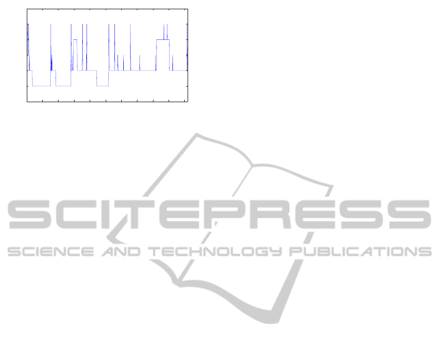
A sample diagram of the distribution and time
evolution of sleep stages, also known as a hypnogram,
is shown in Fig. 1. This hypnogram is one of the
244 polysomnographic recordings used in the present
paper. It consists of 1,020 30-second epochs, which
amounts to 8.5 hours of sleep. Sleep progression gen-
erally starts with the wake stage and then there are
cycles in which REM and NREM alternate, partic-
ularly between REM stage and stage 2. During the
whole night sleep recording, stage 2 exhibits long un-
interrupted bouts as the night goes on. REM episodes
tend to get longer in the second half part of the night
sleep, while stage 3 occurs earlier in the first half of
the night. Finally, there are several times of short
wakefulness throughout the night, after the initial on-
set of sleep. Regardless of these typical patterns of
human sleep, hypnogram details vary across individ-
uals and are affected by age, circadian rhythms (Dijk
and Lockley, 2002), and other factors.
Sleep stage composition is a basic description of
sleep structure that comprises total sleep time, sleep
efficiency, and percentage of sleep period time in each
of the stages within a night of sleep (Khasawneh et al.,
2011). However,these features provide an incomplete
description of human sleep that does not capture the
dynamical information in hypnograms. Sleep stage
duration is widely used in applications to sleep-wake
architecture, where exponential and power-law func-
tions have been proposed as parametric models for
122
Wang C., A. Alvarez S., Ruiz C. and Moonis M..
Computational Modeling of Sleep Stage Dynamics using Weibull Semi-Markov Chains.
DOI: 10.5220/0004252801220130
In Proceedings of the International Conference on Health Informatics (HEALTHINF-2013), pages 122-130
ISBN: 978-989-8565-37-2
Copyright
c
2013 SCITEPRESS (Science and Technology Publications, Lda.)
0 100 200 300 400 500 600 700 800 900 1000
Wake
REM
Stage 1
Stage 2
Stage 3
Time (epochs)
Sleep stage
Figure 1: Sample hypnogram in the present study.
the distributions of the wake and sleep bout durations
(Chu-Shore et al., 2010). Sleep stage transitions are
additional indicators of the dynamics of human sleep.
For example, (Kishi et al., 2008) argues that dynamic
transition analysis of sleep stages is a useful tool for
elucidating human sleep regulation mechanisms.
Markov chains (Rabiner, 1989) have been used
to model the dynamics of sleep stage transitions.
A simple time-homogeneous Markov chain was the
first applied in the sleep domain (Zung et al., 1965).
However, Markov chains (and more generally, hid-
den Markov models) do not model sleep stage transi-
tions accurately, because these models force geomet-
rically distributed stage bout durations for all sleep
stages, contradicting known experimental observa-
tions (e.g., (Chu-Shore et al., 2010) and the present
paper). Semi-Markov chains, a variant of Markov
chains (Rabiner, 1989), are more suitable for describ-
ing sleep stage sequences as they do not assume an
exponential distribution of stage durations (Yang and
Hursch, 1973) and (Kim et al., 2009).
In the present paper, a semi-Markov chain of sleep
stages is considered as a model of human sleep dy-
namics. The hypnograms of 244 human patients are
used to construct a semi-Markov chain on three sleep
stages: wake stage, NREM stage (stage1, stage2, and
stage 3 combined), and REM stage (see section 2.1).
Both sleep stage transitions and the durations of con-
tinuous bouts in each stage are taken into account. To
compensate for the scarcity of bout durations in the
dataset, kernel density estimation is used to smooth
the data (see section 2.2.2). Exponential, power law,
and Weibull density functions are fit to the smoothed
stage bout duration data (see section 2.3). A new met-
ric for evaluating the goodness of fit is introduced and
used to select the best fit (see section 2.3.4). Thor-
ough experimentation identified the Weibull family of
density functions as the best fit for bout durations in
wake, NREM, and REM stages (see section 3.2). This
contrasts with previous reports that bout durations in
these sleep stages follow a simple exponential or a
power law distribution (Kishi et al., 2008).
The resulting semi-Markov chain is presented in
section 3.2. A comparison of this semi-Markov
chain’s equilibrium distribution and bout duration
probability density functions against those of a clas-
sical Markov chain shows the superiority of the
semi-Markov chain model in capturing the statistics
of sleep dynamics (see section 3.3). Furthermore,
hypnograms generated by this semi-Markov model
are more similar to a typical hypnogram in our pa-
tients’ dataset, than are the hypnograms generated by
a Markov chain model (see section 3.4).
2 METHODS
2.1 Human Sleep Data
The dataset used in this paper consists of a total of 244
fully anonymized human polysomnographic record-
ings. They were extracted from polysomnographic
overnight sleep studies performed in the Sleep Clinic
at Day Kimball Hospital in Putnam, Connecticut,
USA. This population consists of 122 males and 122
females, all suffering from sleep problems. The sub-
jects’ ages range from 20 to 85 and their mean value
is 47.9.
Each polysomnographic recording is split into 30-
second epochs and staged by lab technicians at the
Sleep Clinic. Staging of each 30-second epoch into
one of the sleep stages (wake, stage 1, stage 2, stage 3,
and REM) is done by analyzing EEG, EOG and EMG
recordings during the epoch. In this paper stages 1,
2, and 3 are grouped into a non-REM stage, abbrevi-
ated as NREM. This condenses the representation of
the sleep stages to three: Wake, NREM, and REM,
collectively denoted WNR throughout the paper.
2.2 Descriptive Data Features
In contrast with prior work based on sleep compo-
sition features alone (Khasawneh et al., 2011), this
paper directly uses human hypnogram recordings to
capture dynamical features of sleep. The durations
of continuous uninterrupted bouts in individual stages
are natural candidates for the representation of the
hypnogramrecordings. In order to overcome the spar-
sity of stage duration data, kernel density estimation
is applied to smooth these data.
2.2.1 Sleep Stage Bouts and Bout Durations
Sleep stage bouts and bout durations form the basis
of the data representation in this paper. A stage bout
is defined as a maximal uninterrupted segment of the
ComputationalModelingofSleepStageDynamicsusingWeibullSemi-MarkovChains
123

given stage within a given hypnogram. For exam-
ple, the hypnogram in Fig. 1 contains four different
REM stage bouts (note that the REM plateau between
epochs 800 and 900 is interrupted by two brief wake
bouts, thus giving rise to three distinct REM bouts);
also visible are three stage 3 bouts, and many bouts
of other stages. The duration of a sleep stage bout
is defined as the number of epochs which the bout
spans. The frequency of a stage bout duration is the
number of stage bouts of this same duration present in
the hypnogram. The distribution of a stage’s bout du-
rations (that is, the frequencies of different bout dura-
tions for that stage) can be depicted by the distribution
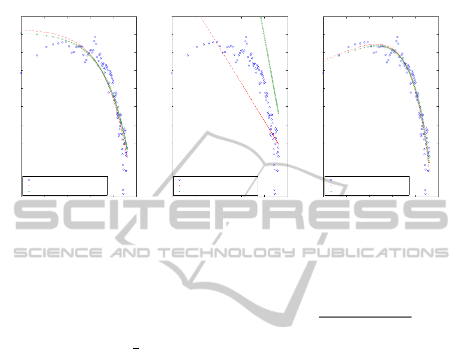
function (probability mass function). A sample distri-
bution of REM stage bout durations over the popula-
tion in the present paper is shown as the data points
on the plots in Fig. 2. As in that figure, stage bout
duration distributions in this paper are calculated over
the entire dataset population, by aggregating bout du-
rations of a given sleep stage (wake, NREM, or REM)
over the 244 individual hypnograms.
2.2.2 Kernel Density Estimation
Kernel density estimation (KDE) is used for nonpara-
metric probability density estimation. It is a useful
statistical smoothing technique used when inferences
about the population are to be made based on a finite
data sample. The stage duration distributions calcu-
lated over our dataset of 244 patients contains many
missing values for specific bout durations in each
sleep stage. KDE is used to smooth these data dis-
tributions, thus providing meaningful values for du-
rations of wake, NREM, and REM stages. A normal
distribution with a kernel-smoothingwindow width of
1 was determined to produced the best results. All ex-
periments were performed in MATLAB
R
(The Math-
Works, 2012). The resulting kernel density estima-
tion for the REM stage is depicted by the circular data
points on the plots in Fig. 2.
2.3 Curve Fitting
Once the stage duration distributions have been
smoothed using non-parametric kernel density esti-
mation as described in section 2.2.2, parametric func-
tions that closely approximate the shape of these du-
ration distributions can be found. (Chu-Shore et al.,
2010) and (Kishi et al., 2008) have shown that good
approximations to stage bout duration distributions
can be obtained by using single exponential func-
tions and power law functions. In this paper, in ad-
dition to single exponential and power law functions,
Weibull functions are considered as candidate fitting
functions. The approach described in section 2.3.5 is
followed for finding optimal parameter values and se-
lecting the best fitting function for each sleep stage
probability density distribution. A newly defined
goodness of fit criterion described in section 2.3.4 is
used to guide this selection. All curve fitting experi-
ments were performed in MATLAB.
2.3.1 Exponential Density Function
The general form of a single exponential distribution
is given in equation 1, where µ is the expected value.
f(x;µ) =
1
µ
exp
−x
µ
(x ≥ 0) (1)
Range of Initial Values for Parameter Estimation.
The expected value of the exponential distribution for
a given sleep stage in MLE corresponds to the ex-
pected value of durations over the sleep stage data.
In this paper, the maximum length of stage bout dura-
tion for all sleep stages is 230 epochs. Therefore, the
initial values for µ can be taken to be between 1 and
230.
2.3.2 Power Law Density Function
The general form of a power law distribution is given
in equation 2.
f(x;α, x
min
) =
α− 1
x
min
x
x
min
−α
(x ≥ x
min
) (2)
The estimation of α in the power law distribution us-
ing maximum likelihood estimation is shown in equa-
tion 3.
α = 1+ n
"
n
∑
i=1
ln
x
i
x
min
#
(x
i
≥ x
min
α > 1) (3)
Range of Initial Values for Parameter Estimation.
According to the estimation in equation 3, and based
on the hypnogram dataset, x
min
should be 1, and a
large enough range for initial values for α is the range
from 1 to 10 times the MLE estimate of α. A delta
increment value of 0.01 is used to select sufficient α
values in this range. Note that n is the number of ob-
served empirical data, namely 244 patients.
2.3.3 Weibull Density Function
The general form of the Weibull distribution is given
in equation 4.
f(x;λ, µ) =
k
λ
x
λ
k−1
exp
−
x
λ
k
(x ≥ 0) (4)
HEALTHINF2013-InternationalConferenceonHealthInformatics
124
0 1 2 3 4 5
−8
−7.5
−7
−6.5
−6
−5.5
−5
−4.5
−4
−3.5
−3
Log Duration
Log Frequency
Exponential Fitting
0 1 2 3 4 5
−8
−7.5
−7
−6.5
−6
−5.5
−5
−4.5
−4
−3.5
−3
Log Duration
Log Frequency
Power Law Fitting
0 1 2 3 4 5
−8
−7.5
−7
−6.5
−6
−5.5
−5
−4.5
−4
−3.5
−3
Log Duration
Log Frequency
Weibull Fitting
Log Duration VS. Log Frequency
LS
ML
Log Duration VS. Log Frequency
LS
ML
Log Duration VS. Log Frequency
LS
ML
Figure 2: Curve fitting of the REM stage duration distribution. The three plots depict the fits obtained by using exponential
functions (left), power law functions (center), and Weibull functions (right). In each plot, the results of the ML and LS
approaches described in section 2.3.5 to find best fits are presented. Among all these candidate fits, the Weibull function
achieves the best goodness of fit, as discussed in section 3.2.3.
where λ is scale parameter and k is shape parameter
in the Weibull distribution. When k = 1, the Weibull
distribution coincides with an exponential distribu-
tion. The expected value of the Weibull distribution
is given by equation 5.
E(x) = λΓ
1+
k
λ
(5)
where Γ is the gamma function, which extends the
factorial function. When k = 1, E(x) = λ.
Range of Initial Values for Parameter Estimation.
To be consistent with the kernel estimated data distri-
bution, k is limited to a range between 0 and 2. λ can
range from 1 to 230 (the maximum duration of any
sleep stage).
2.3.4 Goodness of Fit
A goodness of fit metric is needed to quantify the
discrepancy between data estimated by KDE in sec-
tion 2.2.2 and fitting curves obtained by the above
three fitting functions. This metric can also be used to
select the best among several candidate fitting curves.
A new such metric is introduced below in equation 6,
which is similar to the Mean Square Error (MSE)
metric applied to the logarithmically transformed fre-
quency data, except that the parameter x appears in
the denominator of the new metric. This new metric
proved superior to other metrics (including MSE) in
capturing the quality of the approximation as gauged
by visual inspection during systematic experimenta-
tion.
GOF(x) =
n
∑
k=1
(logs(x
k
) − log f(x
k
))
2
x
k
!
(6)
In equation 6, s(x
k
) refers to the nonparametric prob-
ability density estimation at duration x
k
, and f (x
k
)
refers to the fitting data on s(x
k
). Logarithms are taken
on the estimated data s(x
k
) and fit data f(x
k
) to match
the visual aspect of these values in a log-log scale plot
such as the one in Fig. 2.
2.3.5 Searching for Best Curve Fits
The following approach was employed to search for
the best possible curve fits for each sleep stage dura-
tion distribution (Wake, NREM, and REM).
1. Calculate the stage duration distribution from the
244 hypnograms as described in section 2.2.1.
2. Smooth this stage duration distribution using
KDE as described in section 2.2.2.
3. Fit exponential, power law, and Weibull functions
to the smoothed stage duration distribution using
each of the following two approaches to estimate
parameters:
ML: Use Maximum Likelihood (ML) to estimate
the parameters of each of the fitting function
families. As an illustration, the plots in Fig. 2
depict the best ML approximation obtained for
ComputationalModelingofSleepStageDynamicsusingWeibullSemi-MarkovChains
125

:DNH
15(0 5(0
:DNH:DNH
G3
15(015(0
G3
5(05(0
G3
1
:
D
®
:1
D
®
15
D
®
51
D
®
:5
D
®
5
:
D
®
15(0
G
:DNH
G
5(0
G
Sleep Stage
Wake NREM REM
Wake 0
NREM 0
REM 0
1
:
D
®
:1
D
®
51
D
®
15
D
®
:
5
D
®
5:
D
®
Figure 3: Example of a semi-Markov chain model (SMCM). Similar to a Markov chain model (MCM), a SMCM consists of a
state diagram (which in this case includes three stages: Wake NREM, and REM) together with a transition probability matrix
that provides the probability of transition between each pair of states. The difference between a SMCM and a MCM is that
the probability of a self-transition is made equal to 0 in the SMCM’s transition matrix, and the duration of “staying” in that
state is explicitly represented instead by the probability density function that approximates that stage duration distribution.
the REM stage duration distribution for each of
the three fitting function families.
LS: Use Least Squares (LS) to estimate the pa-
rameters. In this case, the initial parame-
ter values for the estimation were taken from
the ranges described for each function family
(exponential, power law, and Weibull) in sec-
tions 2.3.1-2.3.3. Repeat this for each possible
initial point in the given range. Then use the
GOF metric to select the best estimation ob-
tained for each function family among all those
obtained from the set of initial parameter val-
ues. The plots in Fig. 2 depict the best LS fits
obtained (together with the best ML fits).
4. Use the GOF metric to select the best estimation
obtained by the ML and LS approaches above
across all function families. Output this estima-
tion as the best approximation for the sleep stage
duration distribution.
2.4 Markov Models
Markov models have been extensively used to model
dynamic data. For an excellent survey of Markov
models, see (Rabiner, 1989).
2.4.1 Markov Chain Models (MCM)
A Markov chain model is a particular kind of Markov
model, in which all states are observable (that is, there
are no hidden states). A Markov chain consists of a
collection of states together with a state transition ma-
trix that provides the probability of transition between
each pair of states. The Markov assumption estab-
lishes that this transition probability depends only on
the current state. Markov chains have been used to
model sleep (Zung et al., 1965). However, Markov
chains force exponential state duration distributions,
which is not consistent with known experimental ob-
servations of sleep stage durations (see for instance
Fig. 2). To overcome this limitation, semi-Markov
chain models are investigated in this paper. Markov
chains are used only as a baseline for comparison pur-
poses. Training a Markov chain model over the sleep
data requires only the calculation of the probability
transition matrix over all 244 hypnograms.
2.4.2 Equilibrium Distribution
The equilibrium distribution represents the large-time
asymptotic probability of occupation of the various
states in a Markov chain. Therefore, the equilibrium
distribution characterizes the long-term dynamics of
human sleep in a Markov chain model. The equi-
librium distribution of a Markov chain (but not of a
general semi-Markov chain) may be computed as the
normalized eigenvector of the transition matrix with
eigenvalue 1.
2.4.3 Semi-Markov Chain Models (SMCM)
Different from the Markov chain in section 2.4.1, the
semi-Markov chains as sleep dynamics models have
two components: the stage transition matrix and stage
duration distributions for all stages. The stage transi-
tion matrix is similar to that in the Markov chain ex-
cept that the probability of a transition from any stage
to itself is 0. The best fitting function selected by
section 2.3 should be used as the description of the
stage duration distribution for each stage. The oper-
ation of the semi-Markov chain model is as follows
(see Fig. 3): it starts with a specific stage, usually the
wake stage. The model stays in the current stage for
HEALTHINF2013-InternationalConferenceonHealthInformatics
126

a duration randomly sampled from the duration dis-
tribution for that stage (given by the fitting function
of the stage), expressed as P
Wake
(d
Wake
), after which
time it transitions from the current stage to another
stage selected randomly according to the vector of
stage transition probabilities {a
W→N
a
W→R
}. This cy-
cle is repeated indefinitely.
2.4.4 Equilibrium Distribution Difference
To approximate the equilibriumdistribution in a semi-
Markov chain model, one can use simulation of
the semi-Markov chain. Sufficiently long stage se-
quences are generated so that asymptotic probabili-
ties of states can be estimated. These limiting val-
ues represent the equilibrium distribution of the semi-
Markov chain model.
2.4.5 Fitting Function Difference
In addition to the equilibrium distribution in the semi-
Markov chain model, fitting functions that repre-
sent distributions of stage durations can be compared
throughthe parametervalues if they are from the same
family of functions, for example the Weibull density
function family. Interpreting a sleep bout duration as
a ”time-to-failure” as in statistical reliability theory,
the Weibull distribution indicates a distribution where
the failure rate is proportional to a power of time. The
shape parameter k determines one of several cases: if
k < 1, then failure rate decreases over time; if k = 1,
then it does not change over time; otherwise failure
rate increases with time.
3 RESULTS
3.1 Markov Chain Model
A Markov chain (section 2.4.1) provides a simple dy-
namical model of the transitions between sleep stages.
We discuss the results of constructing a Markov
model over the set of all 244 hypnograms.
3.1.1 Markov Transition Matrix
The resulting transition probability matrix is given in
Table 1. Noticeably, the self–transition probabilities
are much higher than the inter–state transition proba-
bilities.
3.1.2 Markov Equilibrium Distribution
As in section 2.4.2, the equilibrium distribution of
the Markov chain model is obtained by normalizing
Table 1: Stage transition matrix for Markov chain model.
Sleep Stage Wake NREM REM
Wake 0.9207 0.0764 0.0029
NREM 0.0239 0.9705 0.0056
REM 0.0216 0.0108 0.9676
the eigenvalue 1 eigenvector of the Markov transition
matrix. The equilibrium distribution is given in Ta-
ble 2. It characterizes the long-term dynamics of hu-
man sleep as captured by this Markov chain model.
Table 2: Equilibrium distribution for Markov chain model.
Equilibrium Wake NREM REM
Value 0.23 0.64 0.13
3.2 Semi-Markov Chain Model
Semi-Markov models have similar inter-stage tran-
sition behavior to Markov models. But in contrast
with the Markov chain model, the semi-Markov chain
model allows an explicit representation of the stage
duration distributions. We discuss the semi-Markov
model constructed overthe set of 244 hypnograms be-
low.
In contrast with reports by other researchers
(Kishi et al., 2008) that the durations of wake stage,
NREM sleep stage, and REM sleep stage follow
power laws or single exponential distributions, the
work in the present paper suggests that individual
sleep stages are better modeled by Weibull distribu-
tions as shown in Fig. 2 and Fig. 4.
3.2.1 Semi-Markov Transition Matrix
The stage transition matrix obtained for the semi-
Markov chain model is given in Table 3. As discussed
in section 2.4.3, the self-transition probabilities are
0. This matrix can be calculated from the Markov
chain model transition probability matrix by normal-
izing the inter-state probabilities in each row. This
very simple operation produces values that more di-
rectly reveal the relative likelihoods of various inter-
stage transitions.
3.2.2 Semi-Markov Equilibrium Distribution
The model’s empirically observed equilibrium distri-
bution is given in Table 4. It provides the asymp-
totic probabilities of stages over a collection of sim-
ulation runs where the length of simulations ranged
from 1,000 to 1,000,000. The semi-Markov chain
equilibrium distribution in Table 4 is observed to be
very close to that of the Markov chain model shown
in Table 2.
ComputationalModelingofSleepStageDynamicsusingWeibullSemi-MarkovChains
127
0 1 2 3 4 5
−10
−9
−8
−7
−6
−5
−4
−3
−2
−1
Log Duration
Log Frequency
Wake Stage
Log Duration VS. Log Frequency
SMCM
MCM
0 1 2 3 4 5
−7
−6.5
−6
−5.5
−5
−4.5
−4
−3.5
−3
Log Duration
Log Frequency
NREM Stage
Log Duration VS. Log Frequency
SMCM
MCM
0 1 2 3 4 5
−8
−7.5
−7
−6.5
−6
−5.5
−5
−4.5
−4
−3.5
−3
Log Duration
Log Frequency
REM Stage
Log Duration VS. Log Frequency
SMCM
MCM
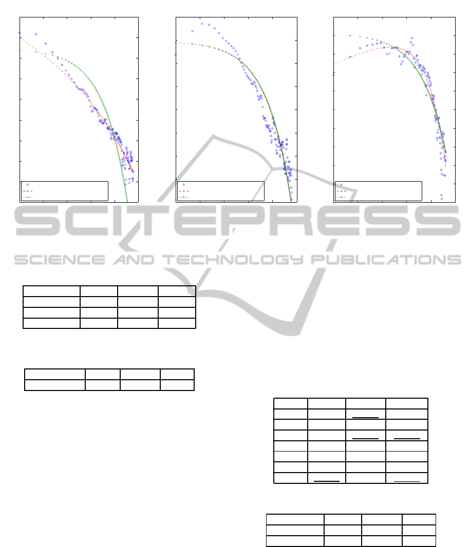
Figure 4: Comparison of fits for the stage duration distribution function used by the Markov chain model (MCM), exponential,
and by the semi-Markov chain model (SMCM), Weibull.
Table 3: Stage transition matrix for semi-Markov chain
model.
Sleep Stage Wake NREM REM
Wake 0 0.9632 0.0368
NREM 0.8093 0 0.1907
REM 0.6655 0.3345 0
Table 4: Equilibrium distribution for semi-Markov chain
model.
Equilibrium Wake NREM REM
Limit 0.25 0.61 0.14
3.2.3 Semi-Markov Stage Duration Model
As a result of the search procedure described in
section 2.3, the Weibull family of distributions was
selected to model the stage durations in the semi-
Markov model. The best fitting parameters were de-
termined as described in section 2.3.5. The results
are summarized in Table 5. It can be seen that for
wake stage, the best fitting function is determined by
least squares error estimation. For NREM and REM,
the best fitting functions are determined by maximum
likelihood estimation. Table 6 provides the param-
eter values for the best Weibull function fits found.
The fact that the Weibull shape parameters for wake,
NREM, REM are, respectively, smaller than, approx-
imately equal to, and larger than 1, show that stage
bout durations for these three stages have character-
istic and distinct behaviors. Specifically, the “failure
rate” for wake, NREM, and REM decreases, does not
change, and increases over time, respectively. These
very different behaviors, which are modeled precisely
in the semi-Markov model, cannot be captured at all
by the Markov model, for which all stage bout du-
rations are exponentially distributed (constant failure
rate, in the reliability metaphor).
Table 5: Goodness of fit (GOF) values, as defined in sec-
tion 2.3.4. The lower this value, the better the fit. The
best fit(s) for each stage is(are) underlined. EDF, PDF, and
WDF denote exponential, power law, and Weibull density
functions, respectively. ML and LS denote the search ap-
proaches described in section 2.3.5.
ML Wake NREM REM
EDF 6.2963 0.5543 1.7284
PDF 2.0704 7.6185 6.0023
WDF 1.0418 0.5684 0.3046
LS Wake NREM REM
EDF 5.0303 0.6352 2.0428
PDF 2.0704 5.8969 11.8552
WDF 0.7788 0.8949 0.3198
Table 6: Parameter values for the Weibull function fits.
Parameters Wake NREM REM
λ (scale) 4.024 33.74 33.35
k (shape) 0.4378 1.000 1.286
3.3 Comparison of Stage Duration Fits
in MCM and SMCM
Fig. 4 depicts for each sleep stage a comparison be-
tween the exponential fit of the sleep stage duration
distribution used by the Markov chain model, and the
Weibull fit used in the semi-Markov chain model. It
HEALTHINF2013-InternationalConferenceonHealthInformatics
128
0 100 200 300 400 500 600 700 800
NREM
REM
Wake
Time (epochs)
Sleep stage
Original hypnogram
0 100 200 300 400 500 600 700 800
NREM
REM
Wake
Time (epochs)
Sleep stage
Generated sequence in semi−Markov chain model
0 100 200 300 400 500 600 700 800
NREM
REM
Wake
Time (epochs)
Sleep stage
Generated sequence in Markov chain model
0 100 200 300 400 500 600 700 800
NREM
REM
Wake
Time (epochs)
Sleep stage
Randomly generated sequence
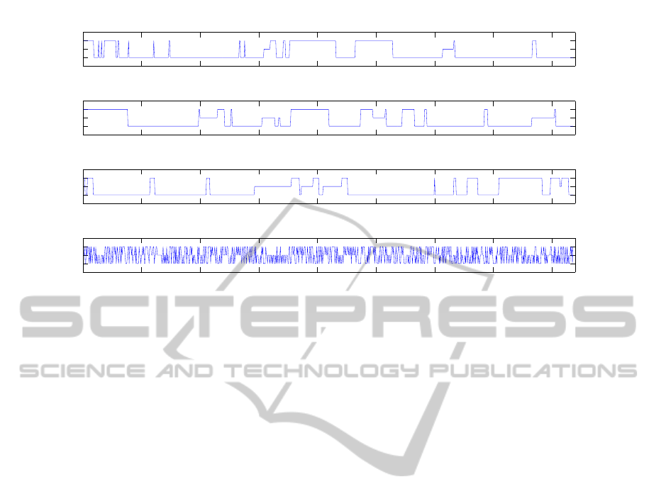
Figure 5: Comparison of an original dataset hypnogram, hypnograms generated by Markov chain and by semi-Markov chain
models, and a randomly generated hypnogram.
can be seen in Fig. 4 that the Weibull funtions used in
the semi-Markov chain model provide a much better
fit for the wake and REM stages than the exponen-
tial functions used by the Markov chain model do.
As examples, the exponential Markov fit underesti-
mates the probability of longer wake bouts, and over-
estimates the probability of shorter REM bouts. The
Weibull semi-Markov fit captures both of these be-
haviors well, by adjusting the shape parameter appro-
priately. The Markov and semi-Markov fits coincide
in the case of NREM, as NREM durations are rela-
tively well modeled by an exponential distribution.
3.4 Comparison of State Sequences
Generated by MCM and SMCM
A comparison between sequences generated by each
the Markov and semi-Markov models, and between
these and the original dataset hypnograms, shed addi-
tional light on the stage transition dynamics captured
by each of the models.
Fig. 5 shows an original dataset hypnogram, sim-
ulated stage sequences generated by the trained mod-
els, and a randomly generated sequence. The ran-
domly generated sequence was obtained by assign-
ing a randomly chosen sleep stage to each epoch us-
ing a uniform distribution over the sleep stages. The
typical hypnogram shown, h, was selected from the
dataset, such that its generative log likelihoods in
the Markov chain model and the semi-Markov chain
model, P(h|MCM) and P(h|SMCM), are close to the
corresponding average log likelihood values over the
entire dataset, which are approximately −148 and
−152, respectively.
Fig. 5 shows, especially near the middle of the
night, that the SMCM better captures the frequency
of both short and long wake durations observed in
the original hypnogram, as compared with the MCM.
This is consistent with the discussion in section 3.3,
in particular Fig. 4. At the onset of the night, the long
uninterrupted duration of wake stage in SMCM sim-
ulates the original hypnogram for the same time pe-
riod better than the short durations of wake stage in
the MCM sequence do. Although MCM is compar-
atively worse than SMCM, its overall distribution of
stages matches the all-night stage composition of the
original hypnogram more accurately than the random
sequence does. This single example is of course in-
tended only as an illustration. The more general anal-
ysis of section 3.3 makes clear the superiority of the
SMCM over the MCM as a model of stage bout dura-
tions, in a robust statistical sense.
4 CONCLUSIONS AND FUTURE
WORK
Widely used Markov chain models of sleep stage
dynamics do not succeed in capturing empirically
observed statistical properties, in particular non-
exponential distribution of certain sleep stage dura-
tions. This paper focuses on the semi-Markov model
in characterizing the dynamics of human sleep stage
bouts and transitions. Unlike a standard Markov
chain model, the semi-Markov model allows describ-
ing the distribution of sleep bout durations indepen-
ComputationalModelingofSleepStageDynamicsusingWeibullSemi-MarkovChains
129

dently from the sequence of stage transitions. This
paper has described the process of constructing semi-
Markov chain models of sleep dynamics, using three
states that represent wake, NREM, and REM stages.
The Weibull family of distributions are empirically
found to faithfully describe the bout durations in these
three stages, providing improved modeling as com-
pared with a standard Markov chain. There are sev-
eral possible directions for future work. Clustering of
hypnograms based on semi-Markov sleep dynamical
models can be considered. The semi-Markov models
with hidden states, analogous to hidden Markov mod-
els, can also be explored. Finally, it is important to
address whether differences in sleep behavior over the
course of one night are adequately described by the
transient (non-equilibrium) behavior of semi-Markov
chains, or if it will instead be necessary to explicitly
incorporate non-stationarity into the dynamical mod-
els.
REFERENCES
Chu-Shore, J., Westover, M. B., and Bianchi, M. T. (2010).
Power law versus exponential state transition dynam-
ics: application to sleep-wake architecture. PloS one,
5(12):e14204.
Dijk, D. J. and Lockley, S. W. (2002). Invited review:
Integration of human sleep-wake regulation and cir-
cadian rhythmicity. Journal of applied physiology,
92(2):852–862.
Khasawneh, A., Alvarez, S. A., Ruiz, C., Misra, S., and
Moonis, M. (2011). EEG and ECG characteristics
of human sleep composition types. Fourth Interna-
tional Conference on Health Informatics (HEALTH-
INF 2011), pages 97–106. Best Paper Award.
Kim, J., Lee, J. S., Robinson, P., and Jeong, D. U. (2009).
Markov analysis of sleep dynamics. Physical Review
Letters, 102(17):178104.
Kishi, A., Struzik, Z. R., Natelson, B. H., Togo, F., and
Yamamoto, Y. (2008). Dynamics of sleep stage tran-
sitions in healthy humans and patients with chronic
fatigue syndrome. American Journal of Physiology-
Regulatory, Integrative and Comparative Physiology,
294(6):R1980–R1987.
Rabiner, L. R. (1989). A tutorial on hidden Markov models
and selected applications in speech recognition. Pro-
ceedings of the IEEE, 77(2):257–286.
Rechtschaffen, A. and Kales, A. (1968). A manual of stan-
dardized terminology, techniques and scoring system
for sleep stages of human subjects. US Department of
Health, Education, and Welfare Public Health Service
- NIH/NIND.
Susmakova, K. (2004). Human sleep and sleep EEG. Mea-
surement Science Review, 4(2):59–74.
Yang, M. C. K. and Hursch, C. J. (1973). The use of a semi-
Markov model for describing sleep patterns. Biomet-
rics, 29(4):pp. 667–676.
Zung, W. W., Naylor, T. H., Gianturco, D. T., and Wilson,
W. P. (1965). Computer simulation of sleep EEG pat-
terns with a Markov chain model. Recent advances in
biological psychiatry, 8:335–355.
HEALTHINF2013-InternationalConferenceonHealthInformatics
130
