Planning of Diverse Trajectories

Jan To

cka, David

ak and Michal P

echou

cek

Agent Technology Center, Department of Computer Science, Czech Technical University in Prague, Prague, Czech Republic

Keywords:

Trajectory Planning, UAV, Human-machine Interface.

Abstract:

Unmanned aerial vehicles (UAVs) are more and more often used to solve different tasks in both the private and

the public sector. Some of these tasks can often be performed completely autonomously while others are still

dependent on remote pilots. They control an UAV using a command display where they can control it manually

using joysticks or give it a simple task. The command display allow for the planning of the UAV trajectory

through waypoints while avoiding no-ﬂy zones. Nevertheless, the operator can be aware of other preferences

or soft restrictions for which it’s not feasible to be inserted into the system especially during time critical tasks.

We propose to provide the operator with several different alternative trajectories, so he can choose the best

one for the current situation. In this contribution we propose several metrics to measure the diversity of the

trajectories. Then we explore several algorithms for the alternative trajectories creation. Experimental results

in two grid domains show how the proposed algorithms perform.

1 INTRODUCTION

Unmanned aerial vehicles (UAVs) are more and more

often used in military operations, in humanitarian and

rescue missions, and in private sector tasks. Some

of the tasks, e.g. the photo-mapping, can often be

performed completely autonomously, while others are

still dependent on remote pilots. They control an UAV

using a command display where they can control it

manually using joysticks or give it a simple task, e.g.

to ﬂy through a sequence of points on the map.

A human operator (pilot) seems to be a bottle-

neck of the system when several UAVs collaborate

on a single mission. Each operator or a team of op-

erators is responsible for one UAV and controls its

actions. The human operators communicate among

themselves and coordinate their actions in order to

achieve a common goal. The whole system contain-

ing UAVs and all HMI machines used to control the

UAVs is called Unmanned Aerial System (UAS). One

of the main goals of research tackling UAVs is to im-

prove the UAS so that a controller or a group of con-

trollers can control larger groups of UAVs easily. This

can be achieved by two means:

• increase UAV autonomy,

• improve human–machine interface (HMI).

In this article we explore a solution which is over-

lapping both of these approaches. It increases the au-

tonomy of UAS as a whole by extension of UAV plan-

ning capability (still not increasing its own autonomy)

and changes the HMI. We will focus on the problem

of the trajectory planning. Usually, all UAVs are con-

trolled directly by remote operators (pilots) or they

can ﬂy following predeﬁned trajectories. In the latter

case, once the operator realizes that a trajectory needs

to be changed, it can deﬁne a new trajectory, e.g. by

means of waypoints and no-ﬂy zones. When the way-

points are updated, the new trajectory is planned (on

UAV or within ground control station). If the operator

agrees with the trajectory it is applied. If the operator

does not want to use the planned trajectory he can re-

ject it and specify a new set of waypoints or introduce

a new no-ﬂy zone to get the trajectory matching his

preferences better.

Even thought the planned trajectory is the optimal

solution with respect to the fuel consumption, needed

time, or other user speciﬁed criteria, the operator can

be aware of other preferences, where the plane should

ﬂy, or soft restrictions on areas which would be nice

to avoid. These can contain, for example, possible fu-

ture colliding trafﬁc, weather conditions, ﬂights over

inhabited areas, etc. It is not feasible to insert all

these preferences into the system, especially during

time critical tasks. The operator typically does not

accept proposed trajectory in the cases when he sees

other which is suboptimal but more preferable one.

Then he has to change input values to force the sys-

tem to give the desired solution. This can be repeated

several times before the trajectory meets all the oper-

120

Toži

cka J., Šišlákand D. and P

echou

cek M..

Planning of Diverse Trajectories.

DOI: 10.5220/0004254601200129

In Proceedings of the 5th International Conference on Agents and Artiﬁcial Intelligence (ICAART-2013), pages 120-129

ISBN: 978-989-8565-39-6

 2013 SCITEPRESS (Science and Technology Publications, Lda.)

Figure 1: New generation of HMI displays will allow a user

to select from several proposed trajectories when the cur-

rent trajectory needs to be replanned. This ﬁgure illustrate

a situation when a new no-ﬂy zone (orange circle) has been

inserted. Since the current UAV trajectory (black colored

stripe) is crossing this new no-ﬂy zone, the trajectory has to

be replanned. Along with the optimal trajectory (cyan tra-

jectory) several alternatives (green trajectory) will be pro-

posed to the user. He can then easily choose new trajectory

based on his own preferences, stay with the current one, or

change the deﬁnition of the trajectory by changing its way-

points or by adding new no-ﬂy zone or removing an existing

one.

ator’s criteria and preferences.

This iterative process can be improved by a system

giving several possible trajectories out of which the

operator selects one based on his preferences which

is then applied. These proposed trajectories should be

different by means of operator perception and prefer-

ences. For example, imagine an UAV ﬂying directly

through a no-ﬂy zone. Shorter way to go around this

no-ﬂy zone is the southern way but the operator sees

that the northern way is just a bit longer and he knows

(based on his experience) that the southern trajectory

can later collide with some other currently unknown

trafﬁc for the planner. Currently used trajectory plan-

ners, e.g. A* (Hart et al., 1968), or Θ* (Nash et al.,

2007), would propose the optimal trajectory, i.e. the

southern one. It can be quite difﬁcult for the opera-

tor to make the UAV to pass around the no-ﬂy zone

by north – he can add an extra way-point or block the

southern direction by new a no-ﬂy zone. At this mo-

ment, it would be very helpful for the operator to have

a possibility to select between the optimal southern

way and an alternative northern way as it’s illustrated

in Figure 1.

It is very difﬁcult to create several plans which are

different enough and understandable from the human

operator’s perspective. Currently there are several al-

gorithms allowing to give k-best solutions but in our

domain all these solution would be usually very sim-

ilar to the best one and can be even indistinguishable

for the human operator. They would typically differ

in a small speed change or in an unobservable devia-

tion from the optimal trajectory. What we really need

are the alternatives which are different from the oper-

ator’s perspective.

The goal of our work is to extend a common tra-

jectory planner so it allows us to create distinguish-

ably different trajectories. Firstly, we need to deﬁne

what different actually means. The notion of differ-

ence is connected to the human perception and thus

can be individual. However, it’s necessary to formally

deﬁne it.

In this contribution we propose several metrics

measuring how much the trajectories differ and sev-

eral approaches to generate different trajectories. We

start with the deﬁnition of several trajectory diver-

sity metrics in Section 2. In Section 3, we describe a

trajectory metric based approach which penalizes the

trajectories similar to the previously generated ones.

Section 4 describes an approach which systematically

extends obstacles and then uses any traditional opti-

mal trajectory planner to ﬁnd individual alternative

trajectories. The last approach, described in Sec-

tion 5, extends this idea by using the Voronoi and the

Delaunay graphs. All the proposed approaches are

evaluated using the presented metrics in two experi-

mental domains and the results are examined in Sec-

tion 6.

For the time being, we focus on a 4-grid and 8-

grid domains (Yap, 2002) and we’ll generalize it to

real coordinates later. We decided to use this domain

because the grid domains are often used as bench-

mark tasks for the trajectory planners. They are often

more complicated than real world domains because

they often contain several optimal paths. Neverthe-

less, proposed algorithms do not change the planners

and thus any planner for more complicated domains

can be used. Figures 2–4 and 6 illustrate which trajec-

tories would be given by each proposed planner in the

4-grid and the 8-grid world with few obstacles (repre-

senting no-ﬂy zones).

Obviously, similar approach can be used in other

real world domains where a system proposes a solu-

tion to a human operator. The operator typically has

broader knowledge about the task and the related en-

vironment. Thus, giving the operator several possibil-

ities can help him to choose the best overall solution.

2 TRAJECTORY DIVERSITY

METRICS

In this section, we introduce several approaches to the

trajectory comparison. We will use deﬁnitions simi-

lar to those used in (Coman and Mu

noz-Avila, 2011),

which deﬁnes the diversity metric for a general plan

PlanningofDiverseTrajectories

121

as follows. Let D : π × π → [0,∞) be a metric de-

scribing the distance between two trajectories. For

a non-empty set of trajectories Π, Coman in (Coman

and Mu

noz-Avila, 2011) deﬁnes the plan-set diversity

Div

(Π) as:

Div

(Π) =

∑

π,π‘∈Π

D(π,π‘)

|Π|×(|Π|−1)

and the relative diversity RelDiv

(π,Π) of plan π rel-

ative to plan-set Π:

RelDiv

(π,Π) =

∑

π‘∈Π

D(π,π‘)

|Π|

where |Π| stands for the number of plans in the plan-

set.

We will use the plan-set diversity to aggregate tra-

jectory distances over the whole set of trajectories.

2.1 Metric: Different States

The different states metric D

States

takes into consider-

ation states of the plans only. In the case of trajectory,

the plan state is the robot location together with some

other attributes, e.g. direction, battery level, etc. In

our experimental domains, the state represents a 2D

location only. Metric D

States

then counts the number

of states of one plan which are also in the other plan

and transforms it into a distance metric:

States

(π,π‘) = 1 −

∑

s∈π

(

1 for s ∈ π‘

0 for s /∈ π‘

|π|

where the |π| stands for the number of states in the

path.

This metric is very general and can be used to

any planning problem, not necessarily to the trajec-

tory planning. In the continuous domain, it would

be useful to add a threshold determining which plane

states are considered to be the same, e.g. based on the

position and heading of the planes.

2.2 Metric: Trajectory Distance

The trajectory distance metric D

Distance

is a general-

ization of the different states metric. It requires some

knowledge about the domain – the distance metric be-

tween the states δ(s

). For each state in the ﬁrst

plan it counts it’s distance to the second plan, i.e. the

distance to the closest state of the other plan.

Distance

(π,π‘) =

∑

s∈π

min

s‘∈π‘

δ(s,s‘)

2.3 Metric: Obstacle Avoidance

The obstacle avoidance metric D

Obstacles

takes also

into consideration how obstacles are avoided by each

trajectory. This idea is based on the human percep-

tion of what are different trajectories. Most of the tra-

jectories well evaluated by the metrics described in

the previous sections are perceived to be very simi-

lar and quite unreasonable – just worsening the op-

timal trajectory without changing anything signiﬁ-

cantly. Human preferred alternatives are often de-

scribed by means of how the obstacles are avoided.

Therefore we need a metric that captures that the ob-

stacles have been avoided from some side. For that we

need to specify what the ’same side’ exactly means.

We say that a robot passes obstacle o by direction d

when a ray going from o in direction d crosses the tra-

jectory. Metric D

Obstacles

is then deﬁned as follows:

Obst.

(π,π‘) = 1−

∑

o∈O

∑

d∈D











1 if π passes o by d

⇔ π‘ passes o by d

0 otherwise

|O||D|

where the O is the set of all obstacles and D is a set of

all directions we are testing. In our experiments, we

use the set of four directions: north, east, south and

west.

3 METRICS BASED PLANNERS

In this section, we introduce a most general ap-

proaches to the trajectory comparison. They are

solely based on the metrics described in Section 2.

This is the most general case which can be easily gen-

eralized to be applied in a general STRIPS planning

problem (Fikes and Nilsson, 1971).

Firstly this planner, listed as Algorithm 1, ﬁnds

the optimal trajectory π

∗

using provided trajectory

planner. Then it iteratively looks for other diverse

trajectories. It updates the goal function to use the tra-

jectory distance metric D together with the current set

of found trajectories Π. The goal function for every

trajectory π is then calculated as the relative diversity

RelDiv

(π,Π).

Let’s have a metric D : π × π → [0, ∞) evaluating

the distance of two trajectories and the relative diver-

sity metric RelDiv(π,Π) as described in Section 2.

We can use it in a planning algorithm to get the next

optimized trajectory which is different enough with

respect to Π trajectories already calculated. This can

easily be done by deﬁning the new evaluating func-

tion

(π) = g(π) + α(MaxDiv − RelDiv

(π,Π)),

ICAART2013-InternationalConferenceonAgentsandArtificialIntelligence

122

Algorithm 1: Trajectory distance metric based di-

verse trajectory planner.

Data: G – state graph

Data: O – set of obstacles

Data: start,target – start and target states

Data: planner – any trajectory planner

Data: n – required number of trajectories

Data: D – trajectory distance metric

Result: Π – set of trajectories

∗

← planner.ﬁndPath(G, O, start,target) ;

Π = {π

∗

} ;

while |Π| < n do

planner.updateGoalFunction(D,Π) ;

π ← planner.ﬁndPath(G,O, start,target) ;

Π ← Π ∪ {π} ;

end

return Π ;

where g(π) is the original price of the trajectory (e.g.

it’s length) and α is the weight of the RelDiv relative

diversity metric value which is transformed into the

penalty by being subtracted from MaxDiv, the maxi-

mal value of the D metric, which is 1 for most of our

cases.

The pro of trajectory based metrics is that, unlike

the other metrics described in the following sections,

they can create different trajectories also for domains

without any obstacles.

3.1 Trajectory Distance Metric Planner

Trajectory distance metric planner uses D

Distance

tra-

jectory distance metric. Trajectories created when us-

ing this metric are very sensitive to the α value. They

can be very suboptimal when the value of α is large.

We can avoid this problem if we omit the trajecto-

ries much worse than the optimal one, e.g. trajecto-

ries more than 20 % longer than the optimal trajectory.

Note that we know the quality of the optimal trajec-

tory because it’s found as the ﬁrst trajectory, before

any metric is used. See Figure 2 for illustration how

the planner with this metric would work.

In our experiments we limit the maximal diversity

value to 2 (MaxDiv in the updated goal function g

All the Div

values bigger than 2 are considered to be

2 and thus result in 0 penalty.

3.1.1 Trajectory Distance Metric MaxMin

Planner

The trajectory distance metric planner tries to mini-

mize the penalty derived from the Div

Distance

diversity

function. That means that it tries to ﬁnd a trajectory,

which is in average the most different to the previ-

ously found trajectories. Another possibility is to look

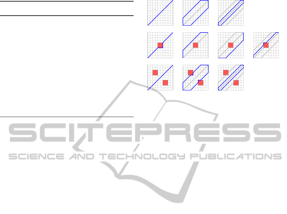
Figure 2: Trajectory distance metric. Blue lines show the

trajectories created during the subsequent runs of the trajec-

tory planner. Dark gray lines show the trajectories forming

the set Π, i. e. the trajectories created during previous it-

erations. We can see that this method is very sensitive to

the threshold specifying how much created trajectory can

differ from the optimal one. In the 2-obstacles case the al-

lowed deviation from the optimal price is not large enough

to cover the cases where the obstacles are passed around.

Note, that even if the algorithm would run more iterations,

such a solution would not be found.

for a trajectory which is the most different to the most

similar trajectory, i.e. to compute the RelDiv

func-

tion as the minimal distance instead of their average:

RelDiv

Min

(π,Π) = min

π‘∈Π

D(π,π‘)

On our illustrative cases, this planner behaves sim-

ilarly to the trajectory distance metric planner (Fig-

ure 2). Nevertheless in our experiments it showed

better performance, especially with respect to the ob-

stacle avoidance metric.

3.2 Different State Metric Planner

The different state metric planner, based on the D

States

metric, is illustrated in Figure 3. We can see that most

of the trajectories are very similar and human opera-

tor would not consider them as real alternatives to the

optimal trajectory.

4 OBSTACLE EXTENSION

APPROACH

This approach works differently than the previous

ones. It transforms the planning task into several new

tasks and then runs a traditional trajectory planner to

ﬁnd the optimal trajectory in each transformed task as

illustrated by Algorithm 2.

PlanningofDiverseTrajectories

123

Figure 3: Different state metric. Blue and dark gray lines

have the same meaning as in Figure 2. It needs several it-

erations to ﬁnd a solution avoiding the 2-obstacles case by

going around – which is better behavior than we observed

in the trajectory distance metric described in Section 3.1.

Algorithm 2: Obstacle extension based diverse tra-

jectory planner.

Data: G – state graph

Data: O – set of obstacles

Data: start,target – start and target states

Data: planner – any trajectory planner

Data: directions – possible extension directions

Result: Π – set of trajectories

∗

← allObstacleExtensions(O,directions) ;

Π = {} ;

forall O

∈ O

∗

π ← planner.ﬁndPath(G,O

,start,target) ;

Π ← Π ∪ {π} ;

end

return Π ;

The transformed task contains obstacles extended

in different directions. Having that each obsta-

cle can be extended to one of 4, or 8, pos-

sible directions, the algorithm tries all possible

combinations of extensions (generated by function

allObstacleExtensions(O,directions)) and for each

combination it takes the shortest trajectory found by

the trajectory planner. This approach is very compu-

tational power demanding – it needs to run the tra-

jectory planner d

-times, where d is the number of

directions, where the obstacles can be expanded, and

k is the number of obstacles. Many cases will result

in the same trajectories or in no solution at all. On

the other hand it allows to create many different al-

ternatives which cannot be found by the previously

described planners. Figure 4 shows how the obstacles

are extended and corresponding trajectories found by

the trajectory planner.

Figure 4: Obstacle extension approach. The blue line is a

trajectory found by the trajectory planner for a task, where

the obstacles are extended in the direction of continuous red

lines. Dashed red lines show other possible obstacle exten-

sions producing the same trajectory. In the 2-obstacles case,

we can see that this approach proposed also a S-shaped tra-

jectory which has not been proposed by any other approach

yet. Even though this trajectory is much longer than the

shortest one and thus would not be probably chosen by the

operator, it well demonstrates that this approach is more

general than the previous ones.

5 VORONOI–DELAUNAY GRAPH

BASED TRAJECTORIES

For each point in the space we can ﬁnd the closest ob-

stacle to that point. Voronoi diagram (Aurenhammer,

1991) is a decomposition of the space into disjunc-

tive Voronoi areas containing points with the same

closest obstacle. The Voronoi graph is composed of

the borders between the Voronoi areas. The edges

represent an abstraction of each passage between the

obstacles. Since this graph is discreet even for 2D

space, it is often used for the trajectory planning (Gar-

rido et al., 2006; Hui-ying et al., 2010). The Delau-

nay graph (Fortune, 1997) is an inverted graph to the

Voronoi graph. The vertexes represent the centers of

Voronoi areas, i. e. the obstacles in our case, and the

edges show which two Voronoi areas have a common

border. For planning alternative trajectories, the algo-

rithm works with the extended Voronoi graph, where

start and target points are connected to the graph. The

Delaunay graph is extended to contain edges connect-

ing centers of outermost Voronoi areas (those which

are crossing the planning area border) towards the

borders

We propose to use the extended Voronoi and the

Delaunay graphs in the problem of ﬁnding diverse tra-

jectories as described in Algorithm 3.

Firstly, the algorithm creates the extended Voronoi

graph G

in the method createExtendedVoronoi-

Graph, which connects also the start and the target

Additional nodes are placed on the intersection of the

border and the added edge into the Delaunay graph.

ICAART2013-InternationalConferenceonAgentsandArtificialIntelligence

124

states

. Then, it ﬁnds all the paths P

from the start to

the target in the extended Voronoi graph G

. For each

path π

, it creates the extended Delaunay sub-graph

where it omits the edges which would cross that

path π

(the method removeDualEdges). The edges

of this new graph G

represent new obstacles. The

method convertEdgesToObsacles converts the edges

of the graph into the obstacle set O

. Then, using any

trajectory planner planner, it ﬁnds the optimal trajec-

tory from the start to the target in the state graph G

avoiding obstacles O and O

Algorithm 3: Voronoi-Delaunay graph based diverse

trajectory planner.

Data: G – state graph

Data: O – set of obstacles

Data: start,target – start and target states

Data: planner – any trajectory planner

Result: Π – set of trajectories

←

createExtendedVoronoiGraph(O,start,target) ;

← ﬁndAllPaths(G

,start,target) ;

Π = {} ;

forall π

∈ P

← createDelaunayGraph(G

) ;

← removeDualEdges(G

,π

) ;

← convertEdgesToObsacles(G

) ;

π ← planner.ﬁndPath(G,O ∪ O

,start,target)

;

Π ← Π ∪ {π} ;

end

return Π ;

The extended Voronoi and Delaunay graphs with

from one iteration of the planning algorithm is

shown in Figure 5. Multiple iterations of the algo-

rithm in the 8-grid domain (Yap, 2002) with few ob-

stacles are shown in Figure 6.

We propose to use the Voronoi and the extended

Delaunay graphs in the problem of ﬁnding different

trajectories as follows. Firstly, we create the Voronoi

graph and extend it by adding borders of the plan-

ning area, which also connects the start and the tar-

get. Then we ﬁnd all the paths from the start to the

target and for each path we create obstacle from the

extended Delaunay graph where we omit the edges

which would cross that path. This new graph contains

original obstacles and their extensions, represented by

the edges, similarly to Obstacle Extension Approach

described in Section 4. Then we just ﬁnd the short-

est path in this new sub-planning problem with any

trajectory planning algorithm. This algorithm is il-

lustrated in Figure 6. This approach is more efﬁcient

than the Obstacle Extension Approach because every

For illustrative purposes we add also a border of the

planning area, but this step is optional.

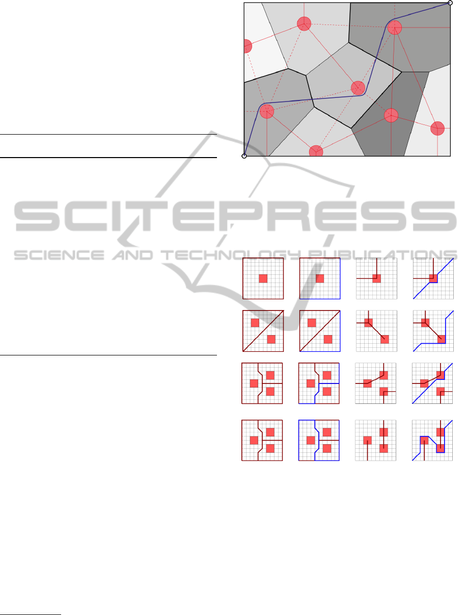
Figure 5: The no-ﬂy zones, represented by the red circles,

deﬁne the Voronoi diagram (gray areas). Its dual graph, the

extended Delaunay graph, is shown by the red lines. When

a path (thicker black line) in the Voronoi graph is found, all

the edges of the extended Delaunay graph, that do not cross

that path, are considered to be the obstacles (continuous red

lines) and the shortest path (blue line) is found using any

optimal trajectory planner.

Figure 6: Voronoi–Delaunay graph based trajectories. Each

row demonstrates subsequent steps of the algorithm. The

ﬁrst column shows the extended Voronoi graph (red lines)

derived from the obstacles. Then all the paths from the start

to the target are found – an example trajectory (blue line)

is shown in the second column. The third column consists

of extended Delaunay graphs (red lines) without the edges

which have been crossed by the current path from the sec-

ond column. Red lines are considered to be obstacles in the

last column, where the alternative trajectory (blue line) is

found by an optimal trajectory planner.

call of the trajectory planner on deﬁned sub-planning

problem will result in a new, original, alternative tra-

jectory.

PlanningofDiverseTrajectories

125

6 EXPERIMENTS

We have evaluated all proposed diverse trajectory

planner in two domains with different number of ob-

stacles. Both domains are based on the 10 × 10 grid

topology, which are often used for the trajectory plan-

ner evaluation: the 4-grid domain which is made of

orthogonal network where each node but the border

ones is connected with 4 neighbors; and the 8-grid do-

main where we allow the diagonal directions too. The

start location is placed to the upper-left corner [0,0]

and the target to the bottom-right corner [10,10]. A

certain number, ranging from 2 to 16, of randomly

generated obstacles are added to each scenario. These

obstacles represent restricted nodes in the grid graph.

During the generation of the obstacles the following

rules had to be fulﬁlled:

1. no two obstacles can be adjacent, and

2. no obstacle can be on the border line, and

3. there exists a path from start to target (implied by

the previous conditions).

These conditions assure that every obstacle can be

avoided by every side and also that there can be a path

between each pair of obstacles. Each run with a given

number of randomly generated obstacles has been re-

peated 10 times and the average value are presented.

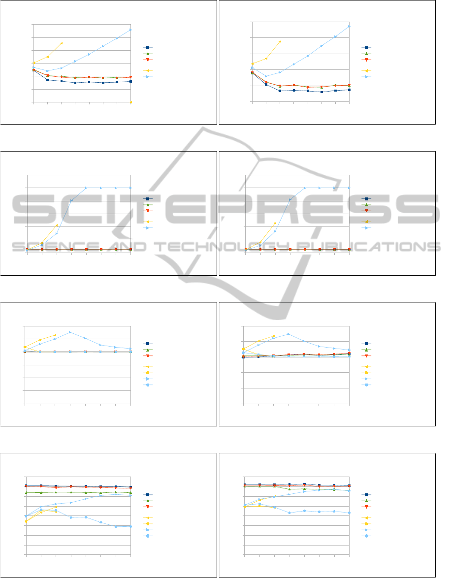
First two graphs (Figures 7 and 8) show how many

alternatives have been found for a different number of

obstacles and how long it took. As expected, values

for the Obstacle extension approach and the Voronoi–

Delaunay graph based approach are growing expo-

nentially with the number of obstacles. The Obsta-

cle extension approach has been evaluated up to 6

obstacles only, since it took too long for the cases

with more obstacles to be evaluated. The computa-

tional complexity of diversity metric based algorithms

is almost constant with a small grow for small num-

ber of obstacles, where the planning algorithm has to

explore larger area before it gets to the target node.

Along with the exponentially growing time complex-

ity of the two algorithms we can see that the num-

ber of found different paths also grows exponentially,

even though it grows only a bit faster for the Obstacle

extension approach, which shows that the Voronoi–

Delaunay graph based approach is more effective.

Since the Voronoi–Delaunay graph based plan-

ner has found too many possible trajectories for even

few obstacles and it would be inappropriate to present

all these trajectories to the user, we decided to limit

the number of evaluated trajectories. Since the main

criteria for the trajectory planning is the trajectory

length, we decided to select 5 or 100 shortest paths

respectively.

The graph in Figure 9 shows the average length

of trajectories given by each planner. And the fol-

lowing graphs (Figures 10–12) show the plan-set di-

versity deﬁned in Section 2 together with one of the

presented trajectory distance metrics.

As expected, the trajectory diversity metric based

algorithms maximized the corresponding metric.

There is one exception in the 8-grid domain with

the trajectory distance metric where, in most cases,

the Voronoi-Delaunay graph based planner had higher

score. This is caused by the limitation of the maximal

distance of trajectories (introduced by the MaxDiv pa-

rameter in the updated goal function) which prevents

creation of trajectories too far from each other.

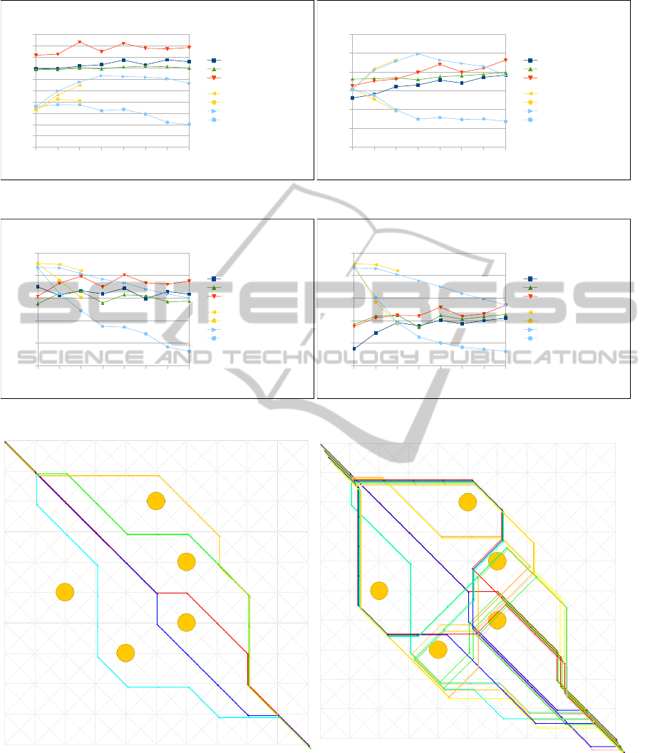
The last Figure 13 shows examples of trajectories

created by the Voronoi-Delaunay graph based diverse

trajectory planner in the scenario with 5 obstacles. We

can see that the 5 shortest trajectories give user a good

selection of different possibilities how to pass the ob-

stacles even though these trajectories were not eval-

uated very well by the presented trajectory diversity

metrics. The reason for that is that even though the

human perception of diversity of trajectories is based

on the trajectory–obstacle relation it is mostly just bi-

nary. Thus if two trajectories avoid any obstacle from

different direction than they are considered to be dif-

ferent. We are now about to proceed with the experi-

ments with human users to verify this hypothesis and,

hopefully, to create a metric which will better reﬂect

human perception.

7 CONCLUSIONS AND FUTURE

WORK

A human-UAV interaction is a bottleneck of today’s

unmanned aerial systems. The interface during the

trajectory planning can be certainly improved by pro-

viding a user with several alternative trajectories from

which the user can choose the most suitable one. This

problem has not been targeted by the scientiﬁc com-

munity yet even though it has a signiﬁcant practical

impact. This contribution introduces the problem of

planning of the alternative trajectories and proposes

several different approaches to its solution.

In the paper, we proposed several ways how to

measure difference of trajectories and also several ap-

proaches to the planning of alternative trajectories it-

self. We started with the trajectory metric based ap-

proaches which penalize the trajectories similar to

the previously generated ones. Then we focused on

the trajectory-obstacles relations and proposed to add

new obstacles into the area to force the planning of

more different trajectories. And ﬁnally we proposed

ICAART2013-InternationalConferenceonAgentsandArtificialIntelligence

126

2 4 6 8 10 12 14 16

0.1

100

1000

10000

100000

Planning Time

Different States Metric Planner

Trajectory Distance Metric

Trajectory MaxMin Distance

Metric Planner

Obstacle Extension - limit (100)

Voronoi-Delaunay - limit (100)

Number of Obstacles

Time [ms]

2 4 6 8 10 12 14 16

100

1000

10000

100000

Planning Time

Different States Metric Planner

Trajectory Distance Metric

Trajectory MaxMin Distance

Metric Planner

Obstacle Extension - limit (100)

Voronoi-Delaunay - limit (100)

Number of Obstacles

Time [ms]

Figure 7: Time.

2 4 6 8 10 12 14 16

100

120

Number of Planned Alternatives

Different States Metric Planner

Trajectory Distance Metric

Trajectory MaxMin Distance

Metric Planner

Obstacle Extension - limit (100)

Voronoi-Delaunay - limit (100)

Number of Obstacles

Number of Alternatives

2 4 6 8 10 12 14 16

100

120

Number of Planned Alternatives

Different States Metric Planner

Trajectory Distance Metric

Trajectory MaxMin Distance

Metric Planner

Obstacle Extension - limit (100)

Voronoi-Delaunay - limit (100)

Number of Obstacles

Number of Alternatives

Figure 8: Number of alternatives.

2 4 6 8 10 12 14 16

Average Trajectory Length

Different States Metric Planner

Trajectory Distance Metric

Trajectory MaxMin Distance

Metric Planner

Obstacle Extension - limit (100)

Obstacle Extension - limit (5)

Voronoi-Delaunay - limit (100)

Voronoi-Delaunay - limit (5)

Number of Obstacles

Trajectory Length

2 4 6 8 10 12 14 16

Average Trajectory Length

Different States Metric Planner

Trajectory Distance Metric

Trajectory MaxMin Distance

Metric Planner

Obstacle Extension - limit (100)

Obstacle Extension - limit (5)

Voronoi-Delaunay - limit (100)

Voronoi-Delaunay - limit (5)

Number of Obstacles

Trajectory Length

Figure 9: Trajectory Length.

2 4 6 8 10 12 14 16

0.1

0.2

0.3

0.4

0.5

0.6

0.7

0.8

Metric: Different States

Different States Metric Planner

Trajectory Distance Metric

Trajectory MaxMin Distance

Metric Planner

Obstacle Extension - limit (100)

Obstacle Extension - limit (5)

Voronoi-Delaunay - limit (100)

Voronoi-Delaunay - limit (5)

Number of Obstacles

Different States

2 4 6 8 10 12 14 16

0.1

0.2

0.3

0.4

0.5

0.6

0.7

0.8

Metric: Different States

Different States Metric Planner

Trajectory Distance Metric

Trajectory MaxMin Distance

Metric Planner

Obstacle Extension - limit (100)

Obstacle Extension - limit (5)

Voronoi-Delaunay - limit (100)

Voronoi-Delaunay - limit (5)

Number of Obstacles

Different States

Figure 10: Different States.

PlanningofDiverseTrajectories

127

2 4 6 8 10 12 14 16

Metric: Trajectory Distance

Different States Metric Planner

Trajectory Distance Metric

Trajectory MaxMin Distance

Metric Planner

Obstacle Extension - limit (100)

Obstacle Extension - limit (5)

Voronoi-Delaunay - limit (100)

Voronoi-Delaunay - limit (5)

Number of Obstacles

Trajectory Distance

2 4 6 8 10 12 14 16

Metric: Trajectory Distance

Different States Metric Planner

Trajectory Distance Metric

Trajectory MaxMin Distance

Metric Planner

Obstacle Extension - limit (100)

Obstacle Extension - limit (5)

Voronoi-Delaunay - limit (100)

Voronoi-Delaunay - limit (5)

Number of Obstacles

Trajectory Distance

Figure 11: Trajectory Distance.

2 4 6 8 10 12 14 16

0.1

0.2

0.3

0.4

0.5

Metric: Obstacle Avoidance

Different States Metric Planner

Trajectory Distance Metric

Trajectory MaxMin Distance

Metric Planner

Obstacle Extension - limit (100)

Obstacle Extension - limit (5)

Voronoi-Delaunay - limit (100)

Voronoi-Delaunay - limit (5)

Number of Obstacles

Obstacle Avoidance

2 4 6 8 10 12 14 16

0.1

0.2

0.3

0.4

0.5

Metric: Obstacle Avoidance

Different States Metric Planner

Trajectory Distance Metric

Trajectory MaxMin Distance

Metric Planner

Obstacle Extension - limit (100)

Obstacle Extension - limit (5)

Voronoi-Delaunay - limit (100)

Voronoi-Delaunay - limit (5)

Number of Obstacles

Obstacle Avoidance

Figure 12: Obstacle avoidance.

Figure 13: Example of trajectories generated by the Voronoi-Delaunay graph based diverse trajectory planner. In the left

ﬁgure we can see the shortest 5 trajectories and all 21 found trajectories are depicted in the right one.

two approaches which systematically extend the ob-

stacles and then use any traditional optimal trajectory

planner to ﬁnd individual alternative trajectories. The

last approach, based on the Voronoi and the Delaunay

graphs, seems to be very promising both in the effec-

tiveness and in the ability to generate many alternative

trajectories. In the time critical scenarios a trajectory

metric based algorithm can be used.

So far, we focused on the 2D grid domains only,

which is often used for the trajectory planners com-

ICAART2013-InternationalConferenceonAgentsandArtificialIntelligence

128

parison. Nevertheless, all the presented algorithms

can be easily generalized to plan in the 3D space.

However, before we start with the deployment of

these methods to a human-machine interface, we need

to evaluate planned diverse trajectories on human op-

erators to choose the most suitable method. This will

form the major part of our future research.

REFERENCES

Aurenhammer, F. (1991). Voronoi diagrams – A survey of a

fundamental geometric data structure. ACM Computer

Survey, 23(3):345–405.

Coman, A. and Mu

noz-Avila, H. (2011). Generating diverse

plans using quantitative and qualitative plan distance

metrics. In AAAI. AAAI Press.

Fikes, R. E. and Nilsson, N. J. (1971). Strips: A new ap-

proach to the application of theorem proving to prob-

lem solving. Artiﬁcial Intelligence, 2(3-4):189–208.

Fortune, S. (1997). Handbook of Discrete and Computa-

tional Geometry, chapter Voronoi diagrams and De-

launay triangulations, pages 377–388. CRC Press

LLC.

Garrido, S., Moreno, L., and Blanco, D. (2006). Voronoi di-

agram and fast marching applied to path planning. In

Proceedings of the 2006 IEEE International Confer-

ence on Robotics and Automation, ICRA 2006, pages

3049–3054. IEEE.

Hart, P., Nilsson, N., and Raphael, B. (1968). A formal

basis for the heuristic determination of minimum cost

paths. IEEE Transactions on Systems Science and Cy-

bernetics, (2):100–107.

Hui-ying, D., Shuo, D., and Yu, Z. (2010). Delaunay graph

based path planning method for mobile robot. In Com-

munications and Mobile Computing (CMC), 2010 In-

ternational Conference on, volume 3, pages 528–531.

Nash, A., Daniel, K., Koenig, S., and Felner, A. (2007).

Theta*: Any-angle path planning on grids. In Pro-

ceedings of the AAAI Conference on Artiﬁcial Intelli-

gence (AAAI), pages 1177–1183.

Yap, P. (2002). Grid-based path-ﬁnding. In Proceedings of

the Canadian Conference on Aritiﬁcial Intelligence,

pages 44–55.

PlanningofDiverseTrajectories

129