Robust 3-D Object Skeletonisation for the Similarity Measure

Christian Feinen

, David Barnowsky

, Dietrich Paulus

and Marcin Grzegorzek

Research Group for Pattern Recognition, University of Siegen, Hoelderlinstr. 3, 57076 Siegen, Germany

Research Group for Active Vision, University of Koblenz-Landau, Universitaetsstr. 1, 56070 Koblenz, Germany

Keywords:

3-D Skeleton Extraction, 3-D Curve Skeletons, 3-D Object Retrieval, 3-D Acquisition and Processing, Human

Perception and Cognition.

Abstract:

In this paper we introduce our approach for similarity measure of 3-D objects based on an existing curve

skeletonization technique. This skeletonization algorithm for 3-D objects delivers skeletons thicker than 1

voxel. This makes an efﬁcient distance or similarity measure impossible. To overcome this drawback, we use

a signiﬁcantly extended skeletonization algorithm (by Reniers) and a modiﬁed Dijkstra approach. In addition

to that, we propose features that are directly extracted from the resulting skeletal structures. To evaluate our

system, we created a ground truth of 3-D objects and their similarities estimated by humans. The automatic

similarity results achieved by our system were evaluated against this ground truth in terms of precision and

recall in an object retrieval setup.

1 INTRODUCTION

Automatic similarity measure of objects is important

for many object recognition systems. One of the most

important similarity features considered by humans is

shape (Pizlo, 2008). Powerful and promising shape

descriptors are skeletons. While skeletonization ap-

proaches in 2-D provide satisfying results (Chang,

2007; Bai and Latecki, 2008), their extensions to 3-D

are lacking of robustness and accuracy. Additionally,

3-D skeletons underlie several constraints: (i) Only

cylindrical geometry delivers curve skeletons; cubes

result in so-called surface skeletons. (ii) The skele-

ton extraction process includes complex mathemati-

cal instruments. (iii) Skeletonization methods require

a high computational effort. Additionally, a plenty

of 3-D approaches for skeletonization deliver skele-

tal structures that are wider than one voxel, e.g., (Re-

niers, 2008). However, skeletons are capable to re-

duce the dimensionality of an object while preserving

important shape characteristics in terms of geometry

and topology.

Although, a plethora of research was done in re-

cent decades, the major amount was dedicated to ob-

tain skeletons and only a little in using them in ob-

ject recognition systems. In this paper we try to

close the gap between extraction and use of skele-

tons as a similarity measure. The signiﬁcant worth of

our work is the constitution of a complete processing

pipeline. Therefore, we employ a skeletonization al-

gorithm proposed by Reniers (Reniers, 2008). Given

the fact that this algorithm does not generate perfect

skeletons, we were forced to extend the Dijkstra al-

gorithm to estimate both, the shortest paths between

skeleton endpoints as well as the location of junction

points within the skeleton. We are aware of the pres-

ence of already existing skeleton extraction methods

that guarantee one voxel wide skeletons, however, Re-

niers’ method produces skeletons with a stable topol-

ogy analogical to the observed object. This prop-

erty has the highest priority for our proposed method,

since we decided to incorporate only topological in-

formation. These features are directly obtained from

the skeletal structure. From a practical point of view,

this decision is reasonable because skeletons are par-

ticularly capable to encode the topological structure

of an object in a highly efﬁcient way. To evaluate our

system, a ground truth of 3-D objects is used whose

similarities are estimated by humans.

Our paper is structured as follows. We start by dis-

cussing relevant existing skeletonization algorithms

for 2-D and 3-D objects (Section 2). Afterwards, Sec-

tion 3 introduces Reniers’ skeletonization method as

well as the improvements made to it within our own

approach. Subsequently, Section 4 describes the pro-

posed similarity measure. In Section 5, we quantita-

tively evaluate our system based on the ground truth

qualiﬁed by humans. Finally, Section 6 concludes our

work and grants a deeper look into upcoming future

tasks.

167

Feinen C., Barnowsky D., Paulus D. and Grzegorzek M. (2013).

Robust 3-D Object Skeletonisation for the Similarity Measure.

In Proceedings of the 2nd International Conference on Pattern Recognition Applications and Methods, pages 167-175

DOI: 10.5220/0004255601670175

 SciTePress

2 RELATED WORK

In the late 1960 Harry Blum introduced an initial

approach for describing objects by skeletons (Blum,

1967) and the well known medial axis (transform) has

been proposed. In subsequent years further methods

have been developed in order to extract skeletons pri-

marily in 2-D. Many of them are mapped into 3-D,

but there are still problems. One of the most popu-

lar methods are Thinning algorithms. This is one of

the most frequently used techniques to generate curve

skeletons of 3-D objects. The idea is to remove iter-

atively the object’s surface (3-D) (or boundary (2-D))

(Pal´agyi and Kuba, 1998; Pal´agyi and Kuba, 1999;

Ma and Sonka, 1996). Voronoi algorithms are also a

popular representative in this domain. The resulting

skeletons are a subset of voronoi edges (Ogniewicz

and Ilg, 1992). Main drawback associated to this type

of algorithms is the high computational complexity.

However, the basic idea was successfully mapped into

3-D space (Ogniewicz and K¨ubler, 1995). 3-D Skele-

tons can also be extracted by the so-called distance

transform methods. We also use this transform in

our system. During the execution of such a method

a distance map is generated that stores the distances

of each location to the closest point on the boundary

or surface (Fabbri et al., 2008; Borgefors, 1996; Re-

niers, 2008). Consequently, all points on the bound-

ary have a zero value. Analogical to the grass ﬁre

ﬂow assumption, this approach implies that skeletal

axes are located at singularities within the distance

map. “Singularities are the points where the ﬁeld is

non-differentiable. When the distance ﬁeld is seen

as a height map, the singularities can be seen as the

mountain ridges and peaks” (Reniers, 2008). Other

techniques employ deformable models (Sharf et al.,

2007) or level sets (Hassouna and Farag, 2007) to

approximate the surface of an object in order to es-

timate curve skeletons. Input of these methods are

point clouds or surface meshes. The output is a thin

and connected 3-D curve skeleton that constitutes a

desired structure in many skeleton-based algorithms.

A further approach which is working on the surface

mesh uses a so-called laplacian-based contraction to

contract the mesh iteratively until it convergesagainst

its centerline (Cao et al., 2010). A good introduction

to the most popular methods is given by the authors

K. Siddiqi and S. Pilzer in (Siddiqi and Pizer, 2008).

There is plethora of different approaches related

to object recognition, but most of them are working

in 2-D. Only less are able to perform directly in 3-D

by using skeletons for a similarity measure. More-

over, talking about 3-D skeleton-based retrieval meth-

ods generally includes both, view-based and model-

based approaches. Since the proposed method be-

longs to the latter, only such algorithms are discussed

in the following. In order to retrieve some informa-

tion about view-based approaches, the work presented

in (Macrini et al., 2002) should be mentioned here.

The authors propose a method where the 3-D model

is represented by a collection of 2-D views. These

views are taken for object recognition using shock

graphs. In (Bai and Latecki, 2008) a 2-D Path Simi-

larity Skeleton Graph Matching approach is presented

which is mapped into 3-D by the authors of (Sch¨afer,

2011). Further techniques based on 3-D skeletal rep-

resentations are introduced in (Cornea et al., 2005)

and (Sundar et al., 2003). As in our work, the authors

of (Cornea et al., 2005) are using the distance trans-

form to generate skeletons. However, in contrast to

our approach, they are using the Earth Mover’s Dis-

tance (EMD) to compute a dissimilarity value. More-

over, such an approach is not suitable for our work

due to the fact that our skeletons are wider than one

voxel.

Apart form this, other competing methods in this

area are based on so-called surface skeletons. In

(Hayashi et al., 2011), e.g., a 3-D shape similarity

measurement technique is proposed which uses sur-

face skeletons of voxelized 3-D shapes. This method

is similar to our approach, but the use of surface skele-

tons can be ambiguous in case of objects consisting of

simple geometry parts and this, in turn, affects the ac-

curacy and robustness of the system. In (Zhang et al.,

2005) a further method to perform 3-D object retrieval

by using surface skeletons is presented. In this work,

the authors place the major focus on the representa-

tion of symmetries of 3-D objects, especially in con-

text of articulated 3-D models.

3 SKELETONIZATION

Reniers used a distance transform to skeletonize 3-

D objects in order to perform segmentation purposes

(Reniers, 2008). These skeletons are wider than one

voxel which, in turn, does not affect his segmentation

approach. In our case, this exacerbates an efﬁcient

computation of distinctive skeleton properties. One-

voxel wide skeletons provide attractive computational

advantages to estimate feature points, e.g., skeletal

junction points. However, the objective of our ap-

proach is to be capable to process these non-perfect, n

voxel wide skeletons (with n ∈ N and n > 1) in order

to guarantee stable and accurate topological informa-

tion. Of course, this includes a thinning procedure

somehow, the detection of end- and junction points,

the estimation of so-called nodal areas, the calcula-

ICPRAM2013-InternationalConferenceonPatternRecognitionApplicationsandMethods

168

tions of geodesics as well as the computation of fea-

ture values. All these points are subject in the Sec-

tions 3.2 - 3.4, whereas Section 3.1 provides a brief

introduction to Reniers’ work.

3.1 Skeleton Extraction According to

Reniers’ Distance Transform

Reniers’ skeleton extraction method is based on a dis-

tance transform. It consists of three steps, namely

(i) the computation of the so-called Tolerance-based

Feature Transform (TFT), (ii) the computation of the

geodesic paths, and (iii) the actual computation of the

skeleton. For each point p inside the 3-D object, the

TFT calculates feature points lying on the object’s

surface. The feature points are computed based on

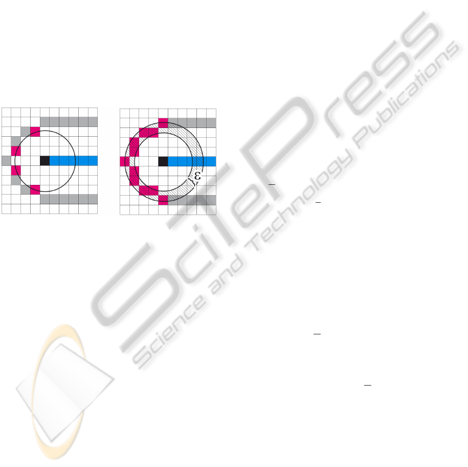
an adjustable tolerance basis as shown in Figure 1.

The TFT was developed in order to handle problems

Figure 1: Working Principle of TFT. The ﬁgure shows the

advantage of using an adjustable tolerance basis (ε) in con-

text of a discretized space. From the top-view of an object

it is clearly noticeable that much more feature points are

detectable by using the TFT.

which occur when the input data has a discretized

structure (volumetric data). As shown in Fig. 2(a),

it is not possible to ﬁnd at least two feature points on

the contour whose lengths are identical to an arbitrary

interior point (black square) inside the rectangle. This

phenomenon is caused by the fact that the number of

voxels is even. In addition to this, it is obvious that

this phenomenon inhibits the estimation of at least

two geodesics between such contour feature points.

Fig. 2(b) shows one of the two possible geodesics

on the contour, please note that the geodesic path to

the opposite side would increase the number of vox-

els by two. These problems are avoidable by adding a

new parameter to adjust a tolerance threshold. Thus,

we are able to ﬁnd at least two geodesics as shown

in Fig. 2(c). Moreover, the detection of at least two

geodesic paths grants us the possibility to detect so-

called Jordan curves and this, in turn, enables us to lo-

cate the desired skeleton points. The actual estimation

of geodesics between all feature points is performed

by using a Dijkstra algorithm. Unfortunately, this cal-

culation is the most time consuming step within Re-

niers’ algorithm. The computation of the tolerance-

based feature transform is not trivial, please refer (Re-

niers and Telea, 2006) to obtain detailed information

about it. According to the formal deﬁnition, a point p

belongs to the skeleton set, if condition (1) is satisﬁed.

Here, Γ indicates the set of all geodesics between the

feature points. More precisely, a point p is part of the

skeletal structure, if it holds a Jordan curve.

p ∈S ⇔|Γ| ≥ 2 (1)

The concrete estimation of Jordan curves are a bit

more complicated as described here. Please refer (Re-

niers, 2008) for a detail description. The result skele-

ton has several drawbacks related to our purpose: (i)

The skeleton is wider than one-voxel. (ii) Junction

points are not exactly deﬁned due to the use of the

TFT and (iii) the distances between junction and end-

points are not uniquely calculable. The Listing be-

low illustrates the explanations above based on some

pseudo code lines in order to grants a deeper under-

standing of this technique.

1: compute feature transform F on Ω

2: for each object voxel p ∈ Ω do

3: F ←

x,y,z∈{0,1}

F(p

+ x, p

+ y, p

+ z)

4: Γ ←

a6=b∈F

shortestpath(a,b)

5: if Γ contains a Jordan curve then

6: S ←S∪{~p}

7: else

8: surface skeleton or non-skeleton voxel

9: end if

10: end for

Line 1-3 compute the TFT for each point p inside the

object Ω. Therefore, line 1 processes an ordinary

feature transform and line 3 stores the set of all

feature points F obtained by the TFT according to

the tolerance values (here: x, y,z ∈ {0,1}).

Line 4 computes the set of geodesics Γ. The

geodesic paths are calculated between all features

points which are stored in F.

Line 5-9 investigate the set of geodesics Γ generated

above in order to detect possible Jordan curves.

These curves can be generated by at least two

geodesic paths. If this is the case, the currently

observed point p is moved to the set of skeleton

points (Eq. 2, where S indicates the set of skele-

ton points).

S ← S∪p (2)

Robust3-DObjectSkeletonisationfortheSimilarityMeasure

169

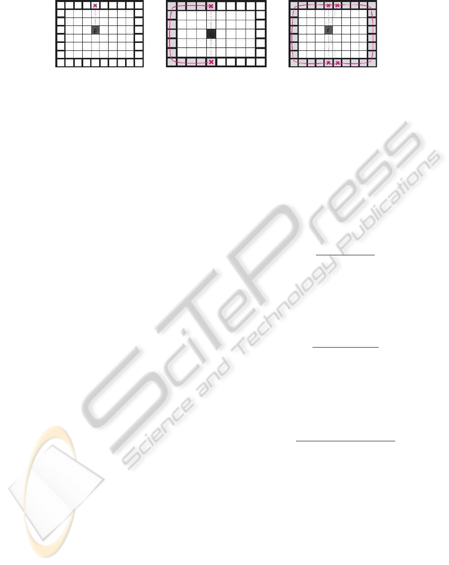
(a) (b) (c)

Figure 2: Problems occurring by using a discretized space. 2(a) shows the problematic to ﬁnd the center line of the rectangle

due to the even number of interior points. Connected to this problem, 2(b) ﬁgures out that the estimation of geodesics is

inhibited as well. 2(c) illustrates the special handling of this problem by using the TFT.

3.2 Skeleton Feature Set

With respect to the problems stated in the previous

section, some modiﬁcations of the skeletal structure

are necessary in order to derive an adequate feature

set. These modiﬁcations are subject of Sec. 3.3

and 3.4. However, in order to modify the skeletons

generated by the algorithm stated above, considera-

tions about an adequate similarity measure have to

be made initially. This means, the feature set has to

be highly compatible regarding both, discrimination

power and consistency to structure changes. Conse-

quently, this vector strongly correlates to the modiﬁ-

cations of the skeleton structure. Thus, we added the

following three constraints to our deliberations. First,

we only incorporate topological information which

are directly obtainable from the skeletal structure

without considering geometrical information (which

could be derived from the 3-D object as well). Actu-

ally, this aim makes it very challenging to discrimi-

nate our objects. However, it perfectly ﬁgures out the

strength of using skeletons to describe articulated ob-

jects. It also demonstrates the robustness of our mod-

iﬁcations made to the skeletons. Second, the features

have to be invariant to rotation, translation and scal-

ing which is an obvious and signiﬁcant advantage for

comparing objects in 3-D. Third, the computation of

our feature set should be fast in order to speedup the

proposed method. That makes it practical for many

applications.

This section introduces the proposed feature vec-

tor. As already mentioned, the feature set is topologi-

cally oriented and includes ﬁve values (Eq. 3).

= (m

)

(3)

Feature 1 indicates the number (m

) of end points

,..., e

. This descriptor reﬂects the complexity

of the object.

Feature 2 is the number (m

) of junction points

,..., n

. This descriptor extends the complexity

value (Feature 1).

Feature 3 describes the mean number of outgoing

paths of a junction point. This can be regarded as

a distribution factor between all end- and junction

points. The higher the value the more endpoints con-

nect to the same junction point on average. The func-

tion c(n

) is a binary function. It returns the value

one, if there is a connection between the endpoint e

and the junction point n.

∑

i=1

∑

j=1

c(n

)

(4)

Feature 4 determines the mean distance of all

skeletal paths (between endpoints). This value en-

codes the lengths of all object segments to one value.

∑

i=1

∑

j=i+1

d(e

)

/2∗(m

−1)

(5)

Feature 5 represents the variance of all shortest

path lengths. This value indicates the regularity of

lengths inside the different object parts.

∑

i=1

∑

j=i+1

(d(e

) −m

)

/2∗(m

−1)

(6)

3.3 Preprocessing

In order to obtain a feature vector as introduced in

Sec. 3.2 minimal demands on end- and junction

points have to be satisﬁed. These requirements con-

cern both, outlier removal and consistency of the

skeleton structure. This became obvious during our

work, as we observed some instability caused by out-

liers as well as by problems regarding the skeleton

structure (stated in Sec. 3.1). Hence, one major point

is the modiﬁcation of Reniers’ skeletons with respect

to the skeletal structure. This issue is debated in Sec.

3.4. In this section we brieﬂy discuss the outlier re-

moval which constitutes only a small part within our

ICPRAM2013-InternationalConferenceonPatternRecognitionApplicationsandMethods

170

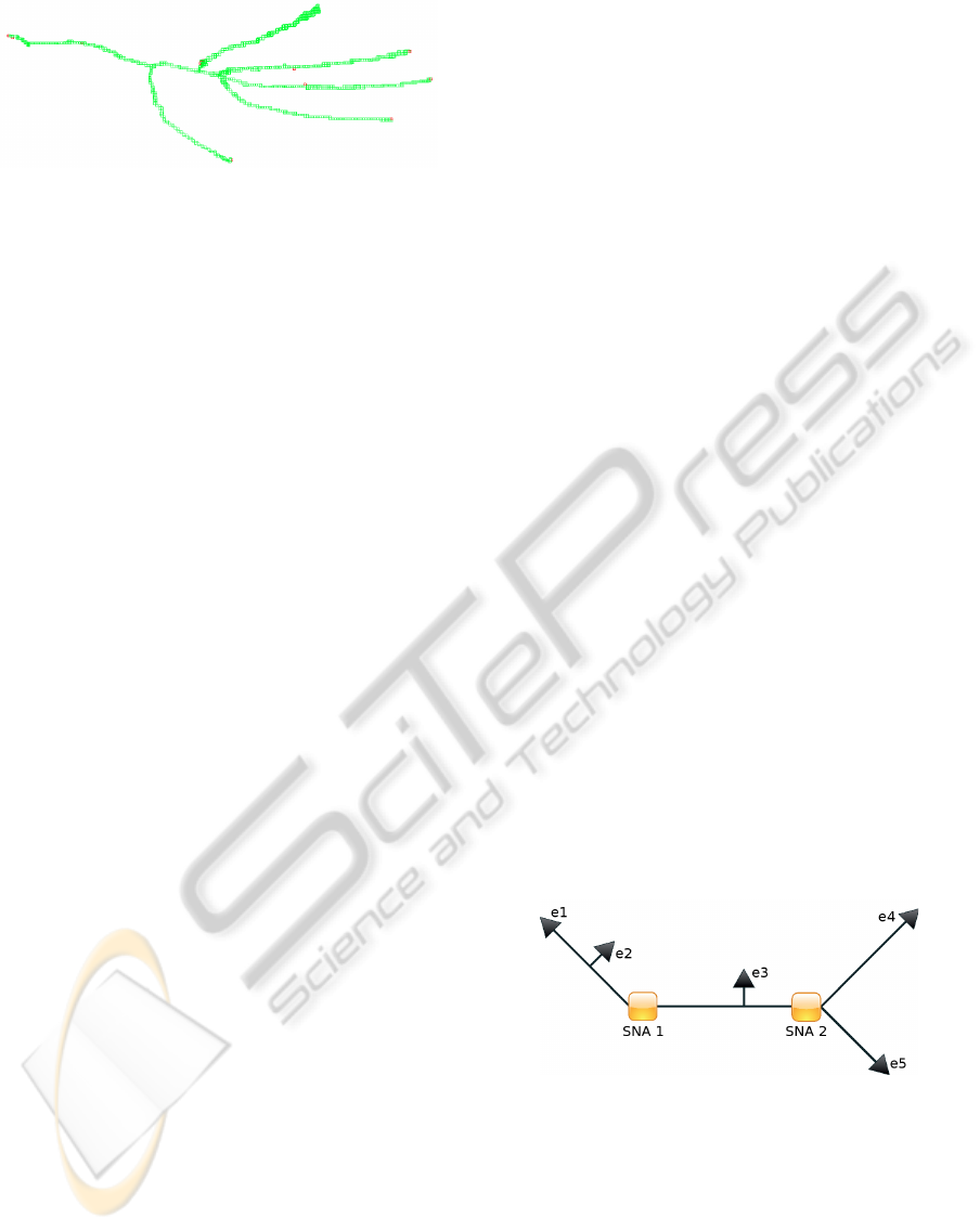
Figure 3: The ﬁgure shows a skeleton after the preprocess-

ing step. The preprocessing is based on morphological op-

erations. In this case a 3 ×3×3 cube is used to perform a

dilatation followed by an erosion.

whole processing pipeline. Therefore, we employ

well-known state-of-the-art methods form the image

processing domain, e.g., thinning and morphological

operators. Since the skeleton extraction method is

time consuming, we tried to employ computationally

attractive techniques to speedup the whole process-

ing pipeline. tasks. In order to evaluate each method,

we directly visualized their results with OpenGL. This

was not much effort due to the fact our the dataset

is easily manageable. Thereby, we observed that the

best results are achieved with morphological opera-

tors even we are running the risk that they do not com-

pulsorily preserve the skeleton’s topology structure.

In our case a dilatation followed by an erosion is per-

formed. For both operations, we use a structure ele-

ment (cube) of size 3×3×3. The topological changes

caused by this combination of structure and structure

element are not able to inﬂuence our method nega-

tively. They also outperformed thinning algorithms.

In this way 60% to 70% of all wrong voxels could be

eliminated on average. The remaining 30% are un-

critical since our algorithm is able to handle such an

amount of outliers. Figure 3 shows a skeletons after

the preprocessing step.

3.4 Modiﬁed Version of the Dijkstra

Algorithm

This section describes our ﬁnal approach. As stated

above, there are still outlier voxels. They do not

affect the proposed method negatively since our al-

gorithm will remove them as well during its execu-

tion. In addition to this, it detects the skeleton junc-

tion points and computes the values of our feature

vector. Therefore, we propose the Dijkstra-Skeleton

algorithm (DSA) as a modiﬁed version of the well-

known Dijkstra algorithm. Since the DSA consists

of multiple steps, we will provide an overview about

its operating principle below. Summarized, we bene-

ﬁt from two signiﬁcant advantages by using this new

version. First, we are able to compute our feature

vector. Second, as already stated, we get rid of the

remaining wrong endpoints.

1. The skeleton structure is mapped to a continuous

graph. This means all voxels are transformed into

an adjacency matrix. This matrix stores the dis-

tances between these nodes.

2. Expansion of skeleton nodes to skeleton nodal ar-

eas (SNA). SNAs are sets of points adjacent to

skeleton junction points which are thicker than

one voxel inside the skeleton. They are necessary

to prevent miscalculations of shortest paths. This

can happen, if the original skeleton junction point

is wider than one voxel. In this case the junction

point runs the risk of being skipped and this, in

turn, would lead to a wrong result. This is highly

crucial because the ﬁrst SNA has to be assigned to

each shortest path that is touched by it. In order to

guarantee this assignment all SNAs have to be de-

tected. Therefore, we utilize a 3×3×3 structure

element.

3. Computation of all shortest paths and storage of

the ﬁrst SNA that is passed during the computa-

tion.

4. Validity check of Dijkstra paths based on two ex-

clusion criteria.

• An endpoint is located between two SNAs.

• Multiple endpoints are connected to the same

SNA and the length of the currently observed

endpoint is not the maximum.

Fig. 4 demonstrates both cases. According to our

exclusion criteria, endpoint e

and e

is removed

from the graph.

5. Computation, normalization and storage of all re-

maining values of our feature vector introduced in

Sec. 3.2.

Figure 4: Conceptual representation of a skeleton graph.

The black arrows e

,.. ., e

indicate the skeleton end-

points and the yellow rectangles SNA1 and SNA2 are skele-

ton nodal areas. By executing the modiﬁed Dijkstra algo-

rithm the endpoints e

and e

are removed.

4 SIMILARITY MEASURE

This section brieﬂy describes the selected similarity

measure that is used to compare two 3-D objects. In

Robust3-DObjectSkeletonisationfortheSimilarityMeasure

171

this work, we employ the well-known cosine angle

as deﬁned in (7). Since we are able to arrange our

features in a vector, this similarity measure, or more

precisely the distance, is highly suitable for our pur-

poses. A further beneﬁt is its normalization power

regarding the vector lengths. In order compare two

objects based on their skeletons, we compute the dis-

tance between their feature vectors.

sim

cos

) =

k∗kf

(7)

In addition to this, we rate the quality of a query

with well-known indicators from the ﬁeld of informa-

tion retrieval, namely recall (completeness) and pre-

cision (accurateness). An small example is shown in

Table 2. In order to be capable to compute these val-

ues, a ground truth (GT) has been generated.

4.1 Ground Truth

The GT consists of totally 14 objects. We know that

this amount of objects is much to less in order to per-

form a comprehensive evaluation. Although there are

some standardized databases consisting of more ob-

jects, they are not useful for our project in this ﬁrst it-

eration. The reason for this is the fact that we want to

investigate relations to the human perception. There-

fore, we used a group of volunteers (consisting of

15 students from different research disciplines) and

asked them to rate the the similarity of each object

pair within our database. Even for a small database

like ours, the similarity of 91 object pairs has to be

rated by a single person. If we would split up this

work, we will run the risk to jeopardize the GT’s con-

sistency. This, in turn, would be dramatically, be-

cause the GT a crucial factor to determine the num-

ber of true positives for every query. That means, the

GT provides the basis to compute the so-called opti-

mal hitting set. Unfortunately, the number of possible

(true) hits is not constant in our case caused by the

way of determining similarity groups. Summarized

we were faced with several problems: First, the ob-

jects belonging to each class are not spread uniformly.

Second, test persons were responsible to cluster our

objects into “similarity groups” according to the hu-

man understanding of similarity. On the one hand,

this data provides a high degree of interesting infor-

mation which is discussed in Sec. 5. On the other

hand, we had to ensure that we do not overload our

volunteers with to many rating tasks. Third, the op-

timal hitting set was estimated by a heuristic as ex-

plained as follows:

1. For each object O

all remaining GT objects are

arranged in a descending order within a list ac-

cording to their corresponding GT similarity val-

ues (s(O

)).

2. Afterwards, we compute all differencesof similar-

ity values as shown in Eq. 8 where d

indicates

the similarity value of an object according to its

list position (v).

∆(d

v+1

) (8)

3. Finally, we detect the position of the fourth largest

delta value (∆) and select all objects above this

row as part of the optimal hitting set (H

An example of the procedure is shown in Table 1.

The decision to use the fourth largest difference as a

threshold is based on empirical observations. Besides

this, the actual rating of similarities, which has been

performed by our volunteers, was unrestricted. Every

test person was free to choose continuously different

perspectives on the objects in order to rate their simi-

larity.

Table 1: Example execution of the proposed heuristic to

select whose objects that build an optimal hitting set H

for

an arbitrary query object O

list s(O

) ∆(d

v+1

) ∆-Position O

∈ H

0.9 - -

√

0.65 0.25 1

√

0.64 0.01 7

√

0.45 0.2 3

√

0.3 0.15 4 x

0.06 0.24 2 x

0.02 0.04 5 x

0.0 0.02 6 x

5 EVALUATION

This section presents the results of the evaluation

based on the proposed method. The objects of our

data set are shown in Fig. 5. Unfortunately, our

database is limited to 14 objects. Nevertheless, these

objects are quite challenging and our results are quite

promising.

As already mentioned in Sec. 4.1, the GT sim-

ilarity information was given by human volunteers.

Admittedly, one of the human characteristics is the

skill to decide similarity on fuzzy degrees and thus

the human perception is not binary. However, our

tests discovered two major things. (i) Expressing this

vagueness in numbers constitutes a challenging job

for humans and this (ii) makes it even harder to ar-

range these values subsequently in a consistent and

uniform distributed way. Latter is also affected by the

circumstance that each person scales this fuzziness

ICPRAM2013-InternationalConferenceonPatternRecognitionApplicationsandMethods

172

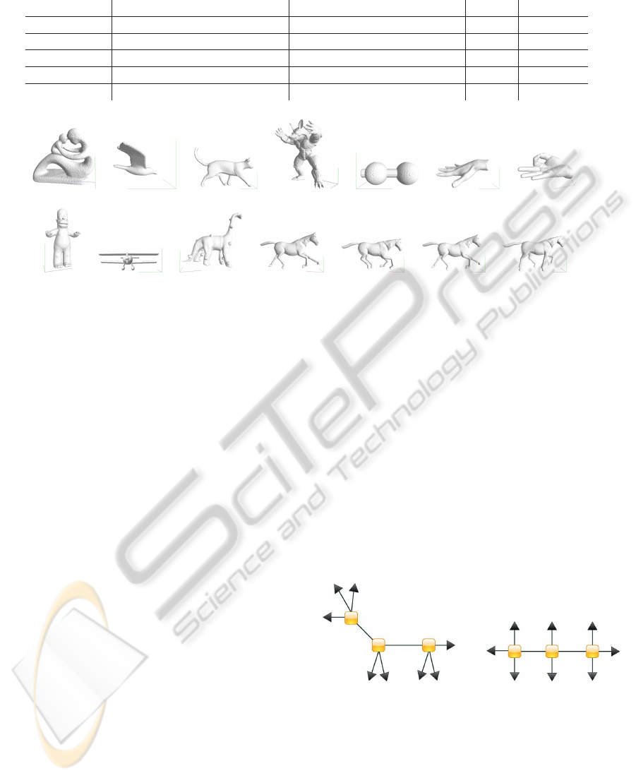
Table 2: Some easy example calculations in terms of Recall and Precision. All content elements are ﬁctitious.

query object optimal #hits (GT) actual #hits (SM) Recall Precision

, O

1 1

, O

0 0

, O

0.5 1

, O

1 0.5

, O

0.5 0.5

(a) o1 (b) o2 (c) o3 (d) o4 (e) o5 (f) o6 (g) o7

(h) o8 (i) o9 (j) o10 (k) o11 (l) o12 (m) o13 (n) o14

Figure 5: Overview about our object database consisting of 14 objects. As shown, most of the objects are articulating.

Articulated objects are highly suitable to work with skeletons.

totally different. In order to handle this gap of per-

ception and capability to express vagueness in values,

we limited this information to two categories: similar

and not similar. Consequently, we lost the possibil-

ity to employ a rational differentiation between these

two quantities. As a result of this, we were forced to

compare between two different scales:

1. an ordinal scaled range obtained by humans and

2. a continuous and metric interval-scaled range de-

rived from our similarity measure.

Working with different scales is hard and excludes a

direct comparison of both values. Thus, the whole

evaluation has to be expressed in terms of similar or

not similar. Additionally, we have to consider a very

interesting and crucial phenomena which we call “un-

conscious background-knowledge”. This means, hu-

mans refer to unconscious relationships between ob-

jects during the similarity rating. For example, it is

not surprising that the object group consisting of Fig.

5(o11) to Fig. 5(o14) obtains a high similarity value.

But in case of the objects of Fig.5(o5), 5(o6) and

5(o7) it is a bit surprising. However, with the knowl-

edge in mind it is replicable. Unconscious knowledge

guides persons to form factual connections. Consid-

ering this information, we evaluated our method. As

already stated, we evaluated the results in terms of re-

call (R) and precision (P). The evaluation results are

shown in Table 4. Altogether, most of the results are

quite promising and it can been assumed that our sys-

tems rates similarity of 3-D objects according to a cer-

tain degree of human perception. Nevertheless, it has

to be remarked that the object group of horses leads to

several outliers and that its result is not as accurate as

expected. Although all horses are found by our algo-

rithm, there are multiple wrong classiﬁed objects. The

problem is associated with the decisions we made in

respect of the proposed feature vector. Since we de-

cided to consider only the topological information of

the objects, the feature vector is not able to discrimi-

nate different objects with similar topology in an ad-

equate way (Fig. 6). A further aspect in context of

our feature vector relates to feature 3. This feature

does not provide strong differences within the range

of its values and consequently there is no additional

information.

(a) Horse (b) Three-man kayak

Figure 6: Two synthetically generated skeletons. The ﬁrst

one could be the skeleton of a horse, the second could be

a three-man kayak. As it is shown, the skeletons are ap-

parently different, but in the case that only their topological

structure is considered, the skeletons are not differentiable

any more.

Robust3-DObjectSkeletonisationfortheSimilarityMeasure

173

Table 3: Overview about the human similarity values between each combination of objects. To simplify the interpretation we

encoded object pairs with a highly rated similarity red and object pairs with low similarity blue.

0,10 -

0,12 0,20 -

0,20 0,07 0,27 -

0,12 0,20 0,13 0,05 -

0,13 0,12 0,15 0,13 0,17 -

0,13 0,11 0,12 0,10 0,17 0,90 -

0,19 0,07 0,40 0,47 0,10 0,20 0,13 -

0,08 0,46 0,07 0,07 0,09 0,07 0,10 0,06 -

0,22 0,07 0,38 0,30 0,07 0,10 0,17 0,17 0,07 -

0,13 0,10 0,61 0,23 0,07 0,07 0,10 0,19 0,07 0,60 -

0,13 0,10 0,60 0,23 0,10 0,07 0,10 0,19 0,07 0,59 0,95 -

0,12 0,10 0,63 0,23 0,10 0,07 0,10 0,19 0,07 0,59 0,95 0,92 -

0,13 0,10 0,60 0,23 0,10 0,07 0,10 0,19 0,07 0,61 0,96 0,96 0,95 -

Table 4: On the left you can see the query object which corresponds to Fig. 5. In the second and third column both set of

objects are arranged, the objects which are classiﬁed as similar by our test persons and the objects retrieved by our similarity

measure. The last to columns show the corresponding Recall and Precision value.

query optimal hitting set (GT) actual hitting set (similarity measure) Recall Precision

, O

0.73 0.89

, O

1.00 0.42

, O

0.50 0.33

, O

0.80 0.50

, O

0.50 0.08

, O

0.29 0.67

, O

0.14 0.50

, O

0.67 0.50

, O

0.40 0.25

, O

1.00 0.13

, O

1.00 0.13

, O

1.00 0.13

, O

1.00 0.13

, O

0, O

, O

1.00 0.11

6 CONCLUSIONS

In this paper we introduce an innovative approach

for 3-D object retrieval based on 3-D curve skele-

tons. Therefore, we employ an already existing skele-

ton extraction technique with several drawbacks in re-

spect to our project. To overcome the most signiﬁ-

cant problems of the resulting 3-D skeletons (e.g., a

curve thickness of more than one voxel), we propose

a modiﬁed version of the Dijkstra algorithm. Ad-

ditionally, we present a new feature set. This fea-

ture set only considers the topological structure of the

skeleton which makes it quite challenging to discrim-

inate objects. We decide to ignore the geometrical

information in order to prove the robustness of skele-

tons. The feature vector, in turn, is combined with

a suitable similarity measure, the cosine angle, that

enables us to evaluate our method. In addition to

this, we generate a ground truth database consisting

of 3-D objects. This database is clustered to “similar-

ity groups” by volunteers. Given these information,

we perform a challenging evaluation showing quite

promising results that justify our research. The evalu-

ation values are expressed in well-known terms from

the ﬁeld of information retrieval. In the future, we

will compare our algorithm to other state-of-the-art

techniques. In this context we are going to use a new

medical 3-D object datasets as well as more compre-

hensive and standardized databases as the McGill 3-D

Shape Benchmark, Princeton Shape Benchmark and

ICPRAM2013-InternationalConferenceonPatternRecognitionApplicationsandMethods

174

objects from the AIM@Shape database. As a result of

this, our method is directly comparable to other meth-

ods. Moreover, since the medical 3-D object database

is already evaluated based on skeletons by using their

geometrical features, we are able to compare these re-

sults against whose of our method. Finally, we are go-

ing to combine both, the topological and geometrical

information. Related to this, we will extend our refer-

ence set (GT) as well and we are going to investigate

other possibilities of 3-D object representation. Fur-

ther research plans consider also other skeletonization

algorithms, features and feature sets as well as other

input data structures (e.g. point clouds, meshes). The

latter point is quite interesting considering the steadily

increasing amount of, e.g., Kinect devices and the

number of research based on such a device. Besides

this, we plan to improve all of our tests in terms of

invariance power and noise sensitivity.

ACKNOWLEDGEMENTS

This work was funded by the German Research Foun-

dation (DFG) as part of the Research Training Group

GRK 1564 “Imaging New Modalities”.

REFERENCES

Bai, X. and Latecki, L. (2008). Path similarity skeleton

graph matching. Pattern Analysis and Machine Intel-

ligence, IEEE Transactions on, 30(7):1282–1292.

Blum, H. (1967). A transformation for extracting new de-

scriptors of shape. In Wathen-Dunn, W., editor, Mod-

els for the Perception of Speech and Visual Form,

pages 362–380. MIT Press, Cambridge.

Borgefors, G. (1996). On digital distance transforms in

three dimensions. Computer Vision and Image Un-

derstanding, 64(3):368 – 376.

Cao, J., Tagliasacchi, A., Olson, M., Zhang, H., and Su, Z.

(2010). Point cloud skeletons via laplacian based con-

traction. In Shape Modeling International Conference

(SMI), 2010, pages 187–197.

Chang, S. (2007). Extracting skeletons from distance map.

International Journal of Computer Science and Net-

work Security, 7(7):213–219.

Cornea, N., Demirci, M., Silver, D., Shokoufandeh, Dick-

inson, S., and Kantor, P. (2005). 3d object retrieval

using many-to-many matching of curve skeletons. In

Shape Modeling and Applications, 2005 International

Conference, pages 366–371.

Fabbri, R., Costa, L. D. F., Torelli, J. C., and Bruno, O. M.

(2008). 2d euclidean distance transform algorithms: A

comparative survey. ACM Comput. Surv., 40(1):1–44.

Hassouna, M. and Farag, A. (2007). On the extraction of

curve skeletons using gradient vector ﬂow. In Com-

puter Vision, 2007. ICCV 2007. IEEE 11th Interna-

tional Conference on, pages 1–8.

Hayashi, T., Raynal, B., Nozick, V., and Saito, H. (2011).

Skeleton features distribution for 3d object retrieval.

In proc. of the 12th IAPR Machine Vision and Appli-

cations (MVA2011), pages 377–380, Nara, Japan.

Ma, C. M. and Sonka, M. (1996). A fully parallel 3d thin-

ning algorithm and its applications. Comput. Vis. Im-

age Underst., 64(3):420–433.

Macrini, D., Shokoufandeh, A., Dickinson, S., Siddiqi, K.,

and Zucker, S. (2002). View-based 3-d object recog-

nition using shock graphs. In Proceedings of the 16

th International Conference on Pattern Recognition

(ICPR’02) Volume 3 - Volume 3, ICPR ’02, pages 24–

28, Washington, DC, USA. IEEE Computer Society.

Ogniewicz, R. and Ilg, M. (1992). Voronoi skeletons: the-

ory and applications. In Computer Vision and Pat-

tern Recognition, 1992. Proceedings CVPR ’92., 1992

IEEE Computer Society Conference on, pages 63–69.

Ogniewicz, R. L. and K¨ubler, O. (1995). Hierarchic voronoi

skeletons. Pattern Recognition, Vol. 28, pages 343–

359.

Pal´agyi, K. and Kuba, A. (1998). A 3d 6-subiteration thin-

ning algorithm for extracting medial lines. Pattern

Recognition Letters 19, pages 613–627.

Pal´agyi, K. and Kuba, A. (1999). Directional 3d thinning

using 8 subiterations. In Proceedings of the 8th Inter-

national Conference on Discrete Geometry for Com-

puter Imagery, DCGI ’99, pages 325–336, London,

UK, UK. Springer-Verlag.

Pizlo, Z. (2008). 3D Shape: Its Unique Place in Visual Per-

ception. The MIT Press, Cambridge - Massachusetts,

London - England.

Reniers, D. (2008). Skeletonization and Segmentation of

Binary Voxel Shapes. PhD thesis, Technische Univer-

siteit Eindhoven.

Reniers, D. and Telea, A. (2006). Quantitative compari-

son of tolerance-based feature transforms. First Inter-

national Conference on Computer Vision Theory and

Applications (VISAPP), pages 107–114.

Sch¨afer, S. (2011). Path similarity skeleton graph matching

for 3d objects. Master’s thesis, Universit¨at Koblenz-

Landau.

Sharf, A., Lewiner, T., Shamir, A., and Kobbelt, L.

(2007). On-the-ﬂy Curve-skeleton Computation for

3D Shapes. Computer Graphics Forum, 26(3):323–

328.

Siddiqi, K. and Pizer, S. (2008). Medial Representations:

Mathematics, Algorithms and Applications. Springer

Publishing Company, Incorporated, 1st edition.

Sundar, H., Silver, D., Gagvani, N., and Dickinson, S.

(2003). Skeleton based shape matching and retrieval.

In Shape Modeling International, 2003, pages 130–

139.

Zhang, J., Siddiqi, K., Macrini, D., Shokoufandeh, A.,

and Dickinson, S. (2005). Retrieving articulated 3-

d models using medial surfaces and their graph spec-

tra. In Proceedings of the 5th international conference

on Energy Minimization Methods in Computer Vision

and Pattern Recognition, EMMCVPR’05, pages 285–

300, Berlin, Heidelberg. Springer-Verlag.

Robust3-DObjectSkeletonisationfortheSimilarityMeasure

175