Evaluating Learning Algorithms for Stochastic Finite Automata

Comparative Empirical Analyses on Learning Models for Technical Systems

Asmir Voden

carevi

, Alexander Maier

and Oliver Niggemann

2,3

International Graduate School Dynamic Intelligent Systems, University of Paderborn, Paderborn, Germany

inIT – Institute Industrial IT, OWL Universitiy of Applied Sciences, Lemgo, Germany

Fraunhofer IOSB – Competence Center Industrial Automation, Lemgo, Germany

Keywords:

Stochastic Finite Automata, Machine Learning, Technical Systems.

Abstract:

Finite automata are used to model a large variety of technical systems and form the basis of important tasks

such as model-based development, early simulations and model-based diagnosis. However, such models are

today still mostly derived manually, in an expensive and time-consuming manner.

Therefore in the past twenty years, several successful algorithms have been developed for learning various

types of ﬁnite automata. These algorithms use measurements of the technical systems to automatically derive

the underlying automata models.

However, today users face a serious problem when looking for such model learning algorithm: Which algo-

rithm to choose for which problem and which technical system? This papers closes this gap by comparative

empirical analyses of the most popular algorithms (i) using two real-world production facilities and (ii) using

artiﬁcial datasets to analyze the algorithms’ convergence and scalability. Finally, based on these results, several

observations for choosing an appropriate automaton learning algorithm for a speciﬁc problem are given.

1 INTRODUCTION

In computer science, the maturing of a ﬁeld of re-

search happens normally in two phases: First, a num-

ber of algorithms are developed. Then in a second

phase, these algorithms are evaluated and compared.

Only after this second phase, their broad application

by non-experts becomes possible. For several rea-

sons, the second phase is often neglected, leaving

non-experts insecure and uneasy about the application

of newly developed algorithms.

The ﬁeld of learning ﬁnite automata, where the

learning includes states and transitions, is an example

for this. Several algorithms have been developed (see

section 3 for an overview), but there is a lack of com-

parative studies. Different algorithms are often evalu-

ated in different application areas, using datasets that

are not always publicly available. Moreover, various

algorithms learn somewhat speciﬁc ﬁnite automata

for which the common comparison criteria have to be

established. This paper will help to close this gap by

introducing several important comparison criteria and

by evaluating algorithms on the same datasets.

In the rest of this section, a motivation for the

learning of automata is given. Section 2 then gives

an overview of stochastic ﬁnite automata formalisms.

Section 3 outlines the four algorithms ALERGIA,

MDI, BUTLA, and HyBUTLA for learning these au-

tomata. Criteria for comparing the algorithms are out-

lined in section 4. In section 5, comparative empiri-

cal analyses are conducted using two real-world pro-

duction facilities. Furthermore, due to the size and

structure limitations of the real datasets, we also use

artiﬁcial data in section 6 for further analyses on the

algorithms’ convergence and scalability. The results

are analyzed in section 7 and observations for the us-

age of these algorithms are given. Section 8 gives a

conclusion.

The learning of automata is a key technology

in a variety of ﬁelds such as model-based develop-

ment, veriﬁcation, testing, and model-based diagno-

sis (Niggemann and Stroop, 2008). The importance

stems from the facts that (i) complex dynamical tech-

nical systems (such as production systems) can be

modeled using different types of ﬁnite automata and

(ii) a manual creation of these models is often too ex-

pensive and labor intensive.

A typical application scenario is the model-based

anomaly detection for technical systems: The more

complex technical system becomes, the more impor-

229

Voden

carevi

c A., Maier A. and Niggemann O. (2013).

Evaluating Learning Algorithms for Stochastic Finite Automata - Comparative Empirical Analyses on Learning Models for Technical Systems.

In Proceedings of the 2nd International Conference on Pattern Recognition Applications and Methods, pages 229-238

DOI: 10.5220/0004255702290238

 SciTePress

Offline learning

Online anomaly

detection

Sensor logs

Learning algorithm

Error

SYSTEM

MODEL

ANOMALY

DETECTION

DATA

Figure 1: Model-based anomaly detection.

tant are automatic and adaptive anomaly detection

and diagnosis systems. This increasing complexity

is mainly due to the high number of software-based

components and the usage of distributed architectures

in modern embedded systems. Ensuring proper func-

tioning of these technical systems has led to the de-

velopment of various monitoring, anomaly detection

and diagnosis techniques. Model-based approaches

have established themselves among the most success-

ful ones. However, they require a behavior model of

a system, which in most cases is still derived manu-

ally. Manual modeling of systems that exhibit state-

based, probabilistic, temporal, and/or continuous be-

havior is a hard task that requires a lot of efforts and

resources. Therefore, researchers have investigated

the possibilities to learn behavior models automati-

cally from logged data (see section 3).

The general approach to model-based anomaly de-

tection, which uses a learned behavior model, is il-

lustrated in ﬁgure 1. In the ﬁrst phase, based on

logs of the system, a model of the normal behavior

is learned. Then, in the second phase, this normal

behavior model is used during a system’s operation

to detect anomalies. For this, the predictions of the

model are compared to the actual measurements from

the running system. If a signiﬁcant discrepancy is de-

tected, the user is informed.

2 FINITE AUTOMATA

FORMALISMS

This paper deals with learning models for the three

types of technical systems: non-timed discrete event

systems, timed discrete event systems, and hybrid

systems. There are many mathematical formalisms

that can model their behavior, e.g. Bond graphs

(Narasimhan and Biswas, 2007), Petri nets (Cabasino

et al., 2010), continuous Petri nets (David and Alla,

1987), hybrid Petri nets (David and Alla, 2001), Par-

ticle ﬁlters (Wang and Dearden, 2009), Kalman ﬁl-

ters (Hofbaur and Williams, 2002) and Bayesian net-

works (Zhao et al., 2005). Due to a number of positive

results for the learning of stochastic ﬁnite automata

from data, they are in the focus of this paper.

Non-timed Discrete Event Systems (nDES) show

a state-based behavior, i.e. they are represented by

a set of discrete states (modes of operation) and a ﬁ-

nite set of events that trigger transitions between those

states (mode switches) (Cassandras and Lafortune,

2008). Such systems can be easily modeled as the

well-known Deterministic Finite Automaton (DFA)

as illustrated in ﬁgure 2(a): States are denoted by s

, s

, and s

, while letters a, b, and c denote events

that trigger transitions. The automaton is determin-

istic in a sense that one event can trigger only one

transition for each state.

(a) Deterministic ﬁnite automaton.

b, p(b)=0.2

a, p(a)=0.8

c, p(c)=0.7

p(s

)=0.2

p(s

)=0.1

(b) Stochastic deterministic ﬁnite automaton.

b, p(b)=0.2

a, p(a)=0.8

=[3,6]

=[1,4]

=[7,14]

c, p(c)=0.7

p(s

)=0.2

p(s

)=0.1

b, p(b)=0.2

θs

a, p(a)=0.8

=[3,6]

=[1,4]

θs

=[7,14]

c, p(c)=0.7

p(s

)=0.2

p(s

)=0.1

(d) Stochastic deterministic hybrid automaton.

Figure 2: Deterministic ﬁnite automata for modeling tech-

nical systems.

Since the behavior of technical systems is always

subjected to statistical ﬂuctuations (e.g. because of

noise or external disturbances), a model should take

this into account. Therefore, a stochastic version of

the DFA was developed (Carrasco and Oncina, 1994).

Stochastic Deterministic Finite Automaton

(SDFA)

Some authors denote such automata probabilistic,

rather than stochastic. E.g. see (Thollard et al., 2000). This

ICPRAM2013-InternationalConferenceonPatternRecognitionApplicationsandMethods

230

is illustrated in ﬁgure 2(b). In contrast to DFA, it mod-

els the probabilities of staying in a state or transiting

to another state given a speciﬁc event.

Technical systems also show a behavior over time,

i.e. timing information must be modeled also. These

systems are called timed Discrete Event Systems

(tDES). In such systems, it is very important at what

particular point in time an event happens. Clearly,

SDFA cannot be used to model tDES. For that reason,

Stochastic Deterministic Timed Automata (SDTA)

are used (stochastic version of timed automaton pre-

sented in (Alur and Dill, 1994)). An example is shown

in ﬁgure 2(c) and, unlike SDFAs, it contains time in-

tervals δ during which transitions must occur.

In addition to state-based, probabilistic and timed

behavior, real-world technical systems also exhibit

a mixture of (value-)discrete and (value-)continuous

behavior over time. So far, the presented formalisms

can only deal with discrete signals (i.e. events). But

within one discrete state, continuous signals often

change their values over time. An example is a ﬂu-

idic system which has two states: First of all, values

such as pressure and ﬂow change over time accord-

ing to one set of differential equations. But if a valve

is opened (the opening corresponds to an event), the

system moves to another state which is described by

a different set of differential equations.

Such systems, where discrete and continuous dy-

namics interact, are called hybrid systems (Alur et al.,

1995; Henzinger, 1996; Branicky, 2005). For model-

ing hybrid systems, the formalism of Stochastic De-

terministic Hybrid Automaton (SDHA) (a stochastic

version of hybrid automaton given in (Alur et al.,

1995)) can be used. A SDHA is illustrated in ﬁg-

ure 2(d): The difference compared to SDTA are the θ

functions associated with discrete states. These func-

tions describe the change of continuous values over

time. A more detailed overview of ﬁnite automata

formalisms can be found in (Kumar et al., 2010).

3 LEARNING STOCHASTIC

FINITE AUTOMATA

3.1 State Merging Approach

In this paper, four well-known automata learning al-

gorithms are presented and evaluated: ALERGIA,

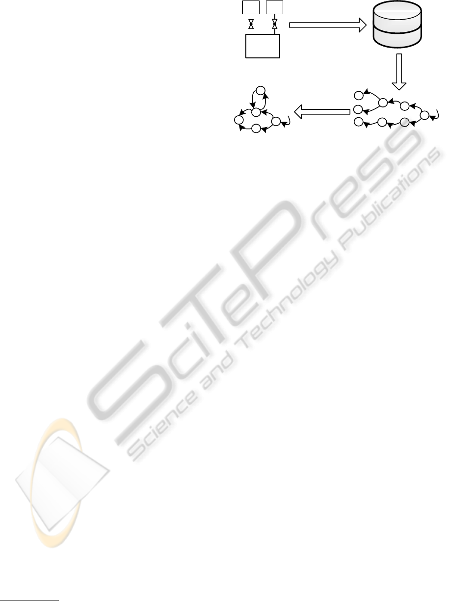
MDI, BUTLA, and HyBUTLA. In general, all these

algorithms use the state merging approach for learn-

ing that is illustrated in ﬁgure 3.

also applies to other types of stochastic automata.

SYSTEM

LEARNED MODEL PREFIX TREE

STEP 1:

System Logs

STEP 2:

Prefix Detection

STEP 3:

State Merging

LOGGED

DATA

Figure 3: State merging approach for learning automata.

In step 1, all relevant signals are measured over

multiple production cycles of system’s normal oper-

ation. Measurements are logged in a database. For

timed systems, logs also include time stamps. For hy-

brid systems, both discrete and continuous signals are

recorded. The underlying data acquisition technolo-

gies are described e.g. in (Pethig et al., 2012).

An initial automaton called Preﬁx Tree Acceptor

(PTA) is then built in step 2. Each logged cycle of a

system represents one automaton learning example.

Each such example comprises multiple events of a

system which are deﬁned as changes in discrete (typ-

ically binary) signals. These changes trigger transi-

tions between automaton states. A PTA is obtained

when common initial sequences of events of differ-

ent examples (i.e. example preﬁxes) are combined to-

gether. A PTA represents different examples as paths

from the initial state to one of the leaf states. Exam-

ples share the preﬁx parts of the paths. So a PTA is

just a smart way to store all examples.

In step 3, the learning takes place: compatible

pairs of PTA states are merged until the underlying

automata is identiﬁed. State merging makes the au-

tomaton smaller and more general. Different algo-

rithms use different compatibility tests.

3.2 Classiﬁcation of Algorithms

In general, the learning algorithms can use learning

examples that can be both positive (coming from a

normal operation) and negative (coming from an ab-

normal operation) (Angluin, 1988). However, in real

technical systems the number of negative examples is

typically very small. Therefore, for the modeling of

technical systems (and in this paper) the focus is on

algorithms relying only on positive examples.

Automata learning algorithms can work either in

an online or an ofﬂine manner (Voden

carevi

c et al.,

2011). Online algorithms can request additional ex-

EvaluatingLearningAlgorithmsforStochasticFiniteAutomata-ComparativeEmpiricalAnalysesonLearningModelsfor

TechnicalSystems

231

amples during the learning process. Ofﬂine algo-

rithms use only a given, static dataset, previously

logged in the system. All four given algorithms de-

scribed in this paper work in an ofﬂine manner.

The order of merging PTA states has a signiﬁcant

inﬂuence on the learning performance, especially the

algorithm runtime (Niggemann et al., 2012). Learn-

ing algorithms normally use either a top-down or a

bottom-up merging order. In the top-down order,

states are checked for compatibility starting from the

initial state and progressing towards the leaf states.

When two states are found to be compatible using

some compatibility measure, their respective large

subtrees have to be recursively checked for compat-

ibility also. This is illustrated in ﬁgure 4 (left), where

subtrees t

and t

have to be compared, before the two

compatible states s

and s

are merged. In the bottom-

up approach (ﬁgure 4 (right)), such recursive checks

are minimized, as the merging process starts at leaf

states and moves towards the initial state. Algorithms

ALERGIA and MDI use the top-down, while BUTLA

and HyBUTLA use the bottom-up merging order.

Figure 4: Top-down (left) and bottom-up (right) merging

orders.

3.3 Learning Algorithms in a Nutshell

Stochastic deterministic ﬁnite automata (SDFAs) can

be learned automatically from data using the algo-

rithms ALERGIA and MDI. Stochastic determinis-

tic timed automata (SDTAs) are learned using the

BUTLA algorithm, while HyBUTLA learns stochas-

tic deterministic hybrid automata (SDHAs). Both

BUTLA and HyBUTLA learn corresponding au-

tomata classes with only one clock for tracking time.

In this section, these algorithms are brieﬂy explained.

The ALERGIA Algorithm. After building a PTA

(see section 3.1), the ALERGIA (Carrasco and

Oncina, 1994) algorithm proceeds with checking the

compatibility of states in a top-down order. For every

single state, the probabilities of stopping in that state

or taking a speciﬁc transition to another state are com-

puted based on the number of its arriving, ending and

outgoing learning examples. Let the number of exam-

ples that arrive to state s

be g

, the number of exam-

ples that end in s

be f

(#), and the number of outgo-

ing examples with the event a be f

(a). The outgoing

probability for s

with the event a is then f

(a)/g

while the ending probability is f

(#)/g

. Once these

probabilities are computed, the compatibility between

any two states s

and s

is evaluated using the Hoeffd-

ing bound (Hoeffding, 1963):



−



log





√



. (1)

where (1 −α)

,α ∈ R,α > 0 is the probability that

the inequality is true. Here, f

and f

denote either

the number of outgoing or ending examples for the

states s

and s

respectively, as the Hoeffding bound

is computed for both probabilities. If the inequality

is true, the difference between estimated probabilities

(left side) is larger than a threshold which depends on

α (right side) and the states will not be merged. Oth-

erwise the states are declared as compatible, and then

their corresponding subtrees are also checked. This is

done by recursively evaluating Hoeffding bound for

all states in both subtrees. When states are ﬁnally

merged, the probabilities are recomputed for a new

state. In addition, due to the possible appearance of

non-determinism in a resulting automaton, it is made

deterministic by merging non-deterministic states and

transitions. Reported time complexity of ALERGIA

is O(n

), where n is the size of the input data. Formal

proof of convergence is given for ALERGIA’s version

called RLIPS in (Carrasco and Oncina, 1999).

The MDI Algorithm. In the ALERGIA algorithm,

the compatibility check based on Hoeffding bound

represents the local merging criterion, i.e. the proba-

bilities of two states and their subtrees are compared.

There is no global information that tells how different

is the whole newly obtained automaton from the pre-

vious one (before merging), or from the initial PTA.

Conversely, the algorithm Minimal Divergence Infer-

ence (MDI) takes this information into account. The

MDI algorithm (Thollard et al., 2000) trades off the

minimal divergence of the automaton from the learn-

ing examples and the minimal automaton size. The

states of the PTA A

are checked for compatibility in

the top-down order like in ALERGIA, but the merg-

ing criterion is based on the Kullback-Leibler (K-L)

divergence between two automata (that also represent

probability distributions of learning examples), rather

than on the Hoeffding bound. The K-L divergence

D(A||A

) between automata A and A

is calculated ac-

cording to:

D(A||A

) =

∑

p(x

|A)log

p(x

|A)

p(x

)

, (2)

where x

represents one example used for learning.

Let A

be the temporary automaton obtained by suc-

cessfully merging states of the PTA A

. Further let

ICPRAM2013-InternationalConferenceonPatternRecognitionApplicationsandMethods

232

be a potential new automaton obtained by merg-

ing the states of A

. The divergence increment while

going from A

to A

is deﬁned as:

∆(A

) = D(A

||A

) −D(A

||A

). (3)

The merge of states of A

will be kept if the diver-

gence increment between obtained automaton A

and

is small enough relative to the size reduction. Let

denote the threshold, and |A

| and |A

| the sizes

of automata A

and A

, respectively (the number of

states). Then the compatibility criterion is:

∆(A

)

|−|A

< α

. (4)

If this inequality is true, the states are similar and will

stay permanently merged. Reported time complex-

ity of MDI is O(n

). Although some experiments in-

dicate that MDI signiﬁcantly outperforms ALERGIA

(see e.g. (Vidal et al., 2005)), MDI lacks the proof of

convergence.

Please note that the MDI algorithm needs to do

the merge ﬁrst in order to obtain the new automaton,

which is then compared with the previous one using

the criterion given by (4). In case the criterion is not

satisﬁed, the merge is discarded and the search for the

next potentially compatible state pair proceeds in the

previous automaton. The number of merges reported

in the results in the following sections represents only

those merges that were not discarded.

The BUTLA Algorithm. ALERGIA and MDI pro-

ceed top-down while searching for compatible states.

The BUTLA algorithm (Bottom-Up Timing Learning

Algorithm) ﬁrstly introduces the bottom-up strategy

(Maier et al., 2011). The criterion for the compatibil-

ity check uses the Hoeffding bound (see equation (1))

similar to the ALERGIA algorithm.

Additionally, BUTLA learns the timing of the

system. In a preprocessing step, for each avail-

able event a probability density function (PDF)—

probability over time—is calculated. If the PDF is the

sum of several Gaussian distributions, separate events

are created for each Gaussian distribution. In the pre-

ﬁx tree creation and in the merging step, these events

are handled as different events.

The HyBUTLA Algorithm. The BUTLA algorithm

merging approach and the learning of timing informa-

tion is also applied in the HyBUTLA algorithm (Hy-

brid Bottom-Up Timing Learning Algorithm). Both

of them have the worst case runtime of O(n

) (sub-

quadratic in the average case). They differ only in

two aspects. First, HyBUTLA learns the behavior of

continuous output signals (based on continuous input

signals). For each state of the preﬁx tree, functions

that describe this behavior are approximated, e.g. us-

ing regression (Hastie et al., 2008). When two states

are merged, their portions of continuous data are com-

bined and functions for the newly created state are

learned. The HyBUTLA algorithm is the ﬁrst hy-

brid automata learning algorithm (Voden

carevi

c et al.,

2011). In the experiments presented in this paper, the

regression method used for learning continuous out-

put functions was multiple linear regression with lin-

ear terms.

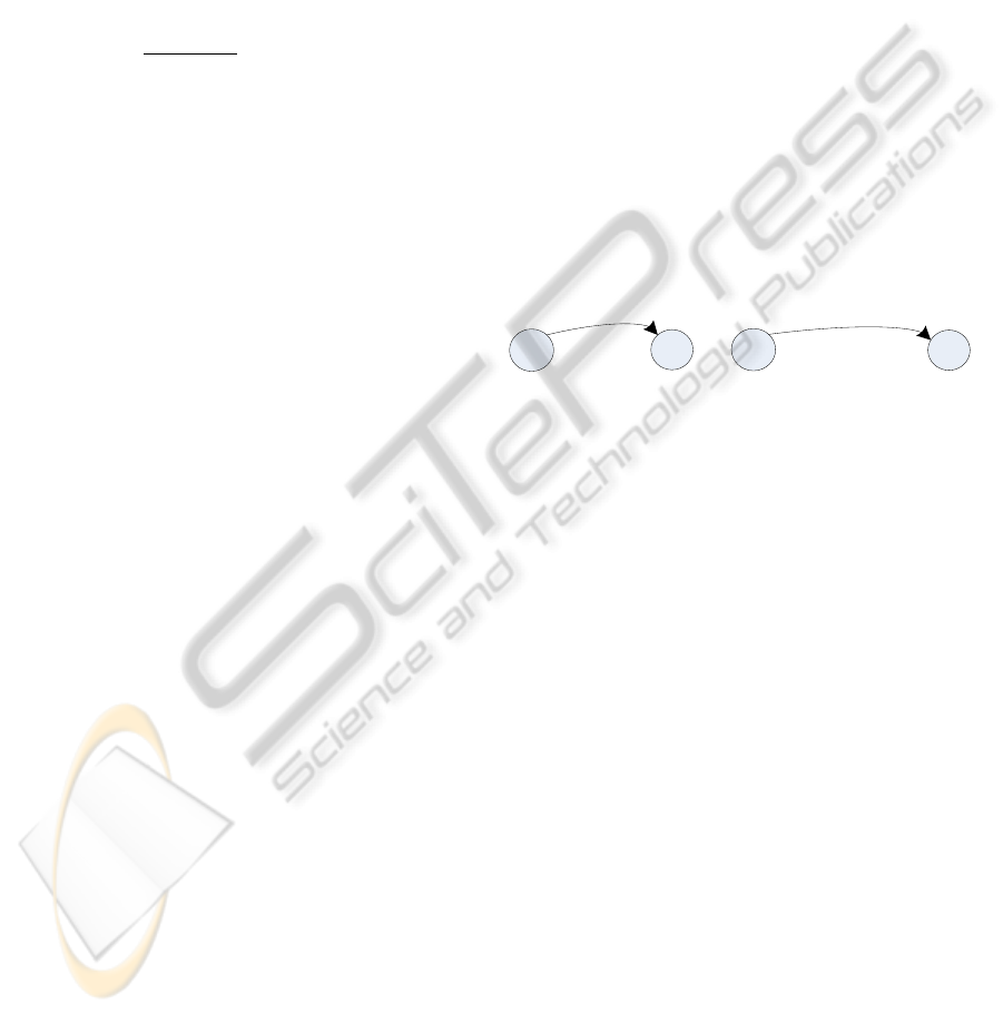
The second difference between HyBUTLA and

BUTLA is that in BUTLA only the status of the

changing discrete signals deﬁnes a transition, while

the status of all other discrete signals is not preserved.

In HyBUTLA, the changing discrete signals also trig-

ger a transition, but the transition event includes the

status of all other discrete signals. This difference is

illustrated in ﬁgure 5. If the system has three discrete

signals: d

, d

, and d

, the change in d

(from 0 to

1) triggers the transition in both algorithms, but the

transition event for BUTLA is deﬁned only as d

= 1,

while for HyBUTLA it contains also values of other

signals: {d

} = {0,1,0}

= 1

} = {0,1,0}

Figure 5: Different event deﬁnitions for BUTLA (left) and

HyBUTLA (right).

4 CRITERIA FOR

ALGORITHM’S EVALUATION

Sections 5 and 6 evaluate the performance of the al-

gorithms using real-world and artiﬁcial data. In this

section, the used criteria and their importance for the

evaluation are outlined.

#states. The number of states is the primary measure

of the automaton size. In general, the goal is to ob-

tain the smallest possible model of a system, with the

highest possible accuracy.

#merges. The number of successful merges tells how

many pairs of states have been merged during learn-

ing. It is closely related to the number of states, as

the sum: (#states + #merges) equals to the number

of states in the preﬁx tree. State merging is used to

reduce the automaton size, but also to make it more

general. Intuitively, the more successful merges, the

higher is the generalization ability of the algorithm.

#comparisons. During a merging step, a search proce-

dure is performed in order to ﬁnd as many compatible

states as possible. The more comparisons are made,

the higher is the chance that compatible states will be

found and merged.

EvaluatingLearningAlgorithmsforStochasticFiniteAutomata-ComparativeEmpiricalAnalysesonLearningModelsfor

TechnicalSystems

233

#determinizations. As stated earlier, some algorithms

use the top-down, while others use the bottom-up

merging order. While merging top-down the large

subtrees are encountered, thus the occurrence of non-

determinism in the automaton is more frequent. Num-

ber of determinizations indicates the portion of non-

determinism created during the merging step, that

needed to be resolved by the learning algorithm.

size reduction (%). Size reduction is the measure

of relative difference between the sizes of the ﬁnal

automaton and the preﬁx tree. It is calculated as

#merges / (#states + #merges). Successful algorithms

can achieve high rates of size reduction.

(%): Averaged coefﬁcient of determination

(%) over the automaton states shows the portion

of variability in the continuous data that is accounted

for by the regression function used for approximation.

Average R

can be measured only for the HyBUTLA

algorithm and it shows its ability to model the con-

tinuous dynamics of the system. In the following ex-

periments, multiple linear regression with linear terms

was used as the regression method.

5 EXPERIMENTS USING

REAL-WORLD SYSTEMS

5.1 The Lemgo Smart Factory

A ﬁrst real-world case study was conducted using an

exemplary plant called the Lemgo Smart Factory at

the Institute Industrial IT in Lemgo, Germany. The

Lemgo Smart Factory is a hybrid technical system

that is used for storing, transporting, processing and

packing bulk materials (e.g. corn). It has a modular

design, uses both centralized and distributed automa-

tion concepts, and comprises around 250 measurable

signals.

Here, the corn processing unit was used as an ex-

ample. In total, logs from 15 production cycles are

available for learning the models. Logs contain the

time stamps, 9 discrete (binary) control signals, 9 con-

tinuous input signals, and machine’s active power as

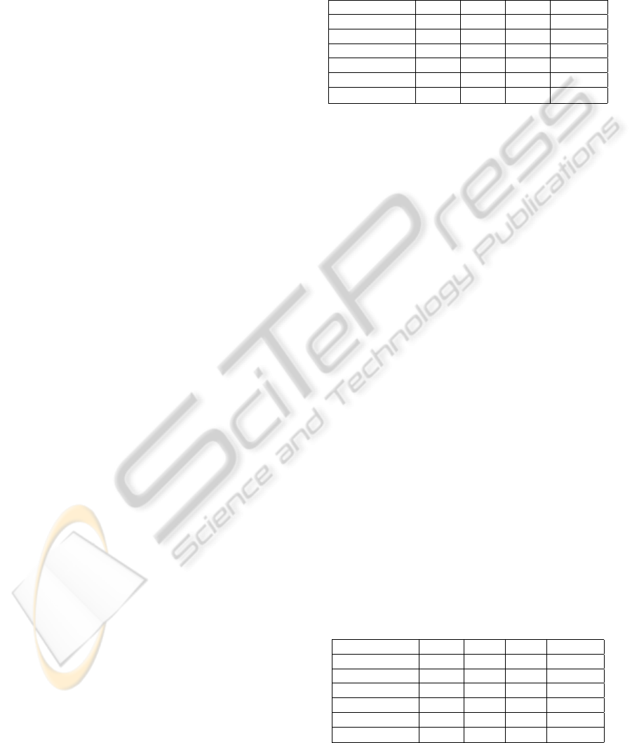
the monitored continuous output variable.

The results are summarized in Table 1. It shows

the values for various comparison criteria outlined in

section 4. On this dataset, the algorithms had similar

performance in the sense of size reduction, number of

states and merges. It can be seen that BUTLA and Hy-

BUTLA performed signiﬁcantly more comparisons

than ALERGIA and MDI. This is due to comparing

the timing of transitions, in addition to comparing

their probabilities. Even with simple method such as

multiple linear regression, high R

value is achieved.

Since ALERGIA and MDI use the top-down merging

order, they had to perform more determinizations.

Table 1: Algorithm comparison for Lemgo Smart Factory

data.

ALE MDI BUT HyBUT

#states 9 13 9 15

#merges 80 76 77 88

#comparisons 130 183 429 733

#determiniz. 44 171 21 14

reduction(%) 89.89 85.39 89.53 85.44

(%) - - - 94.54

5.2 The Jowat AG

The Jowat AG with headquarters in Detmold is one

of the leading suppliers of industrial adhesives. These

are mainly used in woodworking and furniture man-

ufacture, in the paper and packaging industry, the

textile industry, the graphic arts, and the automo-

tive industry. The company was founded in 1919

and has manufacturing sites in Germany in Detmold

and Zeitz, plus three other producing subsidiaries, the

Jowat Corporation in the USA, the Jowat Swiss AG,

and the Jowat Manufacturing in Malaysia. The sup-

plier of all adhesive groups is manufacturing approx.

70,000 tons of adhesives per year, with around 790

employees. A global sales structure with 16 Jowat

sales organizations plus partner companies is guaran-

teeing local service with close customer contact.

The data was logged in one of the plants, dur-

ing production of one product. In total 14 produc-

tion cycles were logged. The modeled part of the sys-

tem is the input raw material subsystem, which con-

tains 6 material supply units (smaller containers) con-

nected to a large container where materials are mixed.

Recorded discrete variables are 15 valve open signals

and their feedbacks (in total 30 discrete variables).

The continuous output variable whose dynamics was

learned is the large container weight. Continuous in-

put variables are weights of 6 smaller containers and

the pressure of the raw material pump. The results of

the algorithms’ comparison are given in Table 2.

Table 2: Algorithm comparison for Jowat AG data.

ALE MDI BUT HyBUT

#states 27 16 17 13

#merges 418 429 473 507

#comparisons 1025 605 4526 3576

#determiniz. 348 578 150 111

reduction(%) 93.93 96.4 96.5 97.5

(%) - - - 89.8

The trends are here similar as in Table 1. High

number of merges and high size reductions are ev-

ICPRAM2013-InternationalConferenceonPatternRecognitionApplicationsandMethods

234

ident for all algorithms. Again, BUTLA and Hy-

BUTLA do more comparisons, while ALERGIA and

MDI perform more determinizations. Also in this

moderately larger system, relatively high R

of around

90 % is achieved.

6 EXPERIMENTS USING

ARTIFICIAL DATA

In this section, learning examples were generated ar-

tiﬁcially from a given input model. This allows (i) for

the generation of arbitrarily complex examples and

(ii) for the assessment of the learned model by com-

paring it to the given input model.

6.1 Convergence Experiments

The experiments given here are conducted to exam-

ine how close the learning algorithms can converge

to the number of states in the predeﬁned model that

generated the learning data. Algorithms use an artiﬁ-

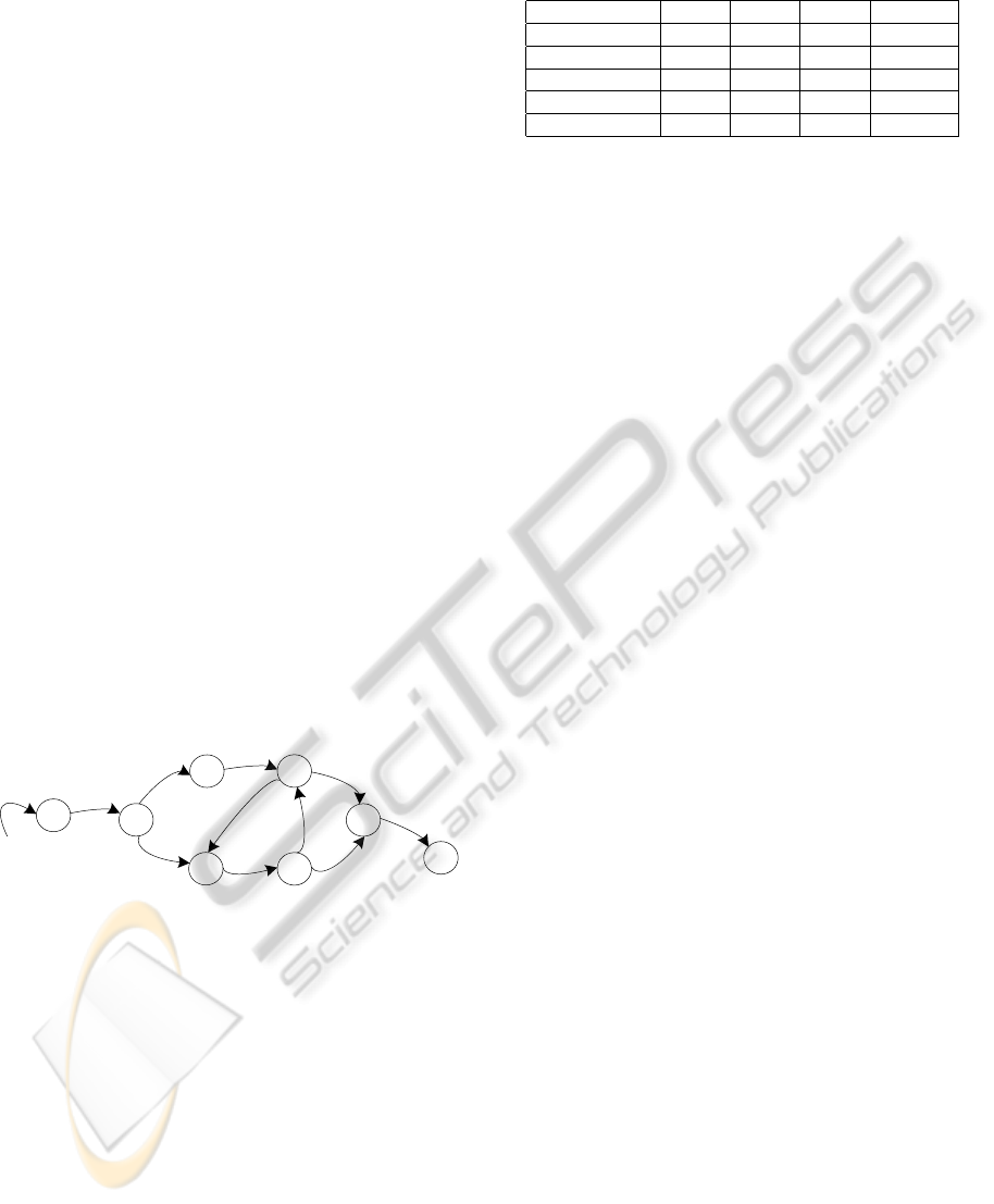
cial dataset randomly drawn according to a predeﬁned

Reber-like model. It is illustrated in ﬁgure 6. Events

that trigger transitions are given together with their

corresponding transition probabilities. The original

Reber model (Reber, 1967) was changed in a way that

equal subsequent events do not occur (including tran-

sitions that have equal source and destination state),

because this cannot appear in production plants.

B(1.0)

T(0.5)

P(0.5)

X(1.0)

V(1.0)

Q(0.5)

S(0.5)

E(1.0)

W(0.5)

Y(0.5)

[7,20]

[1,3]

[4,8]

[4,7]

[2,9]

[10,15]

[8,9]

[6,9]

[7,15]

Figure 6: Reber-like automaton.

The number of generated learning examples was

1000. Example length was around 40 samples. In ad-

dition to discrete variables that trigger transitions (see

ﬁgure 6), one continuous output and ﬁve continuous

input signals were randomly generated according to

normal distribution for HyBUTLA experiments. In-

put and output signals have the mean value and stan-

dard deviation 220 ±22 and 1206 ±120.6, respec-

tively. Moreover, a randomly generated time interval

has been associated with every transition of the au-

tomaton. Summarized results for the four algorithms

are given in Table 3.

indent Due to the different way the HyBUTLA algo-

rithm deﬁnes the transition (see section 3.3), it gener-

ated signiﬁcantly more states in the preﬁx tree, thus

Table 3: Algorithm comparison for artiﬁcial data.

ALE MDI BUT HyBUT

#states 13 5 11 8

#merges 14 22 16 3733

#comparisons 157 43 82 12081

#determiniz. 7 35 1 249

reduction(%) 51.85 81.48 59.26 99.79

having the high number of merges, comparisons, as

well as the high size reduction. However, it converged

to the automaton with the exact number of states of

the Reber-like automaton. ALERGIA had the worst

performance on this task, while MDI and BUTLA had

the same deviation from the target automaton.

6.2 HyBUTLA Scalability Experiments

The goal of scalability experiments is to evaluate the

HyBUTLA algorithm performance, in the presence of

the increasing number of two types of signals in the

system: discrete and continuous. A series of exper-

iments were conducted by increasing the number of

one type of signals, while keeping the number of the

other type constant. Results are given graphically for

created preﬁx tree acceptor (PTA) and learned hybrid

automaton. Given performance metrics include the

number of PTA states, the number of merges, average

model coefﬁcient of determination (R

), size reduc-

tion (in relation to PTA size), and learning time.

In total, 22 artiﬁcial datasets were generated. Each

dataset comprises 10 learning examples. The size of

each learning example was picked from a range of

[150,250] samples with a random number generator

that uses an uniform distribution. Normal distribution

was used for generating independent continuous input

signals, as well as the output signal. The mean value

and standard deviation for input signals is 220 ±22,

and for the output it is 1206 ±120.6. Discrete sig-

nals were generated following an uniform distribu-

tion. They represent independent binary variables.

Locations and lengths of bit-switches are picked ran-

domly for every signal. Each discrete signal changes

two times per learning example. For easier reading,

the number of continuous signals will be denoted by

c, and the number of discrete signals by d.

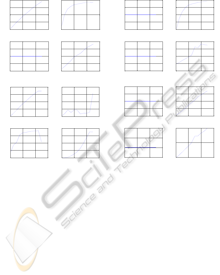
6.2.1 Analysis with Constant Number of

Continuous Signals

In these experiments, d was increased from 1 to 50,

while c was kept constant at value 5. Figure 7(a)

shows the results for PTA. Its number of states in-

creases linearly with d. This makes the portions of

continuous data in each state smaller and easier to

approximate. Therefore, R

rises with d. The re-

EvaluatingLearningAlgorithmsforStochasticFiniteAutomata-ComparativeEmpiricalAnalysesonLearningModelsfor

TechnicalSystems

235

0 20 40 60

200

400

600

800

Number of discrete variables

Number of states

0 20 40 60

100

Number of discrete variables

Average R2 (%)

0 20 40 60

-1

-0.5

0.5

Number of discrete variables

Reduction (%)

0 20 40 60

Number of discrete variables

Learning time (s)

PTA plots for number of continuous variables = 5

#states

reduction(%)

runtime(s)

average R

(%)

#discrete signals d

#discrete signals d #discrete signals d

(a) PTA performance metrics for c = 5.

0 20 40 60

200

400

600

800

Number of discrete variables

Number of merges

0 20 40 60

Number of discrete variables

Average R2 (%)

0 20 40 60

100

Number of discrete variables

Reduction (%)

0 20 40 60

500

1000

1500

2000

Number of discrete variables

Learning time (s)

MERGE plots for number of continuous variables = 5

#merges

reduction(%)

runtime(s)

average R

(%)

#discrete signals d

#discrete signals d #discrete signals d

(b) Learned automaton performance metrics for c = 5.

Figure 7: Results for constant c.

duction is always zero for PTA experiments. PTA

construction time is approximately linear in d. Fig-

ure 7(b) shows results for merged PTAs (learned au-

tomata). The number of merges grows (approxi-

mately linearly) with d. As in the case of PTA, for

higher d, higher R

is obtained. In general, both size

reduction and learning time grow with d. The mea-

sured learning time is subquadratic. Since both PTA

size and the number of merges grow linearly with d

(i.e. with the size of dominantly discrete system), the

size of the ﬁnal learned model will also grow. Ex-

periments are done for more values of constant c, and

the results are similar (not shown due to space restric-

tions).

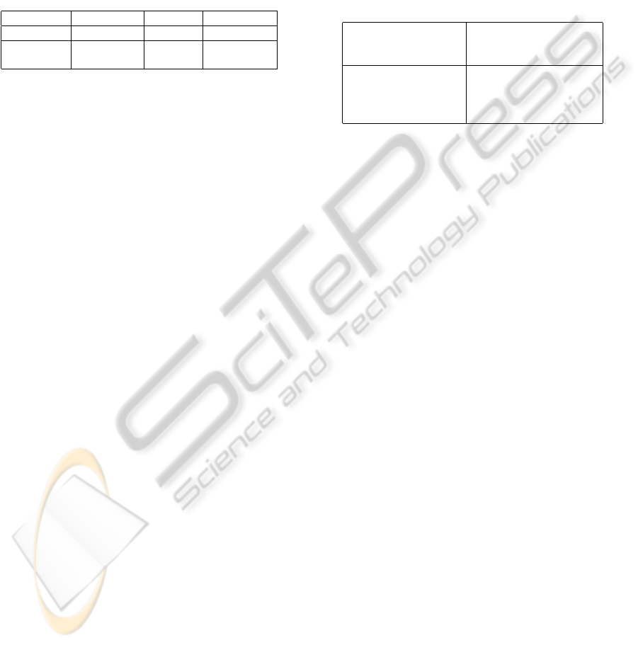
6.2.2 Analysis with Constant Number of

Discrete Signals

Here c was increased from 1 to 50, while d was kept at

value 5. Figure 8(a) gives the results for PTA. Since

states are derived based on changes in discrete sig-

0 20 40 60

88.5

89.5

Number of continuous variables

Number of states

0 20 40 60

100

Number of continuous variables

Average R2 (%)

0 20 40 60

-1

-0.5

0.5

Number of continuous variables

Reduction (%)

0 20 40 60

Number of continuous variables

Learning time (s)

PTA plots for number of discrete variables = 5

#states

reduction(%)

runtime(s)

average R

(%)

#continuous signals c

#continuous signals c #continuous signals c

(a) PTA performance metrics for d = 5.

0 20 40 60

80.5

81.5

Number of continuous variables

Number of merges

0 20 40 60

Number of continuous variables

Average R2 (%)

0 20 40 60

Number of continuous variables

Reduction (%)

0 20 40 60

Number of continuous variables

Learning time (s)

MERGE plots for number of discrete variables = 5

#merges

reduction(%)

runtime(s)

average R

(%)

#continuous signals c

#continuous signals c #continuous signals c

(b) Learned automaton performance metrics for d = 5.

Figure 8: Results for constant d.

nals only, the increase in c does not generate the new

ones. However, the growth of c increases the aver-

age R

. Like before, reduction is zero, while learning

time grows with c. Results for the learned automata

are shown in ﬁgure 8(b). Merging criteria do not in-

clude continuous signals, thus the number of merges

is constant in c (and so is the reduction). Both R

and learning time grow approximately linearly with c.

Since the model size remains unchanged, one should

always try to log and use as many input signals as

possible since more predictors approximate the out-

put signal better. More experiments were conducted

for different values of constant d and similar trends

are observed (not shown due to space restrictions).

7 DISCUSSION

Based on the analysis presented in this paper, several

general observations for learning behavior models for

ICPRAM2013-InternationalConferenceonPatternRecognitionApplicationsandMethods

236

technical systems are given. These observations could

be used in practice by non-experts. Table 4 gives the

overview of stochastic automata formalisms suitable

for modeling the three types of technical systems:

non-timed Discrete Event System (nDES), timed Dis-

crete Event System (tDES), and a Hybrid System

(HS). Table also gives the algorithms that can success-

fully learn such automata.

Table 4: Systems, models and learning algorithms.

System nDES tDES HS

Model SDFA SDTA SDHA

Algorithm

ALERGIA

BUTLA HyBUTLA

MDI

Analyses in real-world systems have shown sim-

ilar trends for smaller exemplary Lemgo Smart Fac-

tory and moderately bigger Jowat AG datasets. It can

be observed that all four algorithms achieved similar

and relatively high size reduction rates in both cases,

which demonstrates their ability to produce small and

more general models. Obtained models that have 9–

27 states can be easily visualized, understood and in-

terpreted by humans, thus they provide a good insight

in the system’s modes of operation and its behavior

in general. Getting such insight by using the pre-

ﬁx trees with hundreds of states would not be possi-

ble. It should be noted that the HyBUTLA algorithm

was able to create models with average R

of around

90% for both systems using relatively simple regres-

sion method such as multiple linear regression. These

models represent the continuous dynamics of the sys-

tems quite well. Furthermore, it can be seen that the

bottom-up algorithms (BUTLA and HyBUTLA) per-

form more thorough search for compatible states, as

they make more comparisons of the states. Intuitively,

this advantage is payed with their increased runtime.

Top-down algorithms create more non-determinism

in the model that they need to resolve.

The convergence experiments on artiﬁcial data

given in section 6.1 have demonstrated that the algo-

rithms can converge either to the exact or close to the

number of states of the predeﬁned model that gen-

erated the learning data. Since most real-world pro-

duction systems are hybrid systems, a special atten-

tion was devoted to the HyBUTLA algorithm in sec-

tion 6.2. Based on the conducted experiments with

changing number of discrete (d), and continuous (c)

signals, further observations are derived and summa-

rized in table 5. For dominantly discrete systems, one

can expect to obtain large PTAs, but at the same time

to beneﬁt from merging in the sense of size reduc-

tion. Very small models (high reduction rates) could

be obtained. Unfortunately, this typically produces

lower accuracy of approximating continuous output

signals (low average R

). For dominantly continuous

systems, the situation is converse. With smaller d,

PTAs of the small size are obtained. Larger c does

not inﬂuence neither the PTA size, nor the number of

merges. Small d enables very few or no merges, thus

merging does not bring signiﬁcant beneﬁt in modeling

such systems in the sense of size reduction. However,

typically higher average R

values can be obtained.

Table 5: Observations for modeling hybrid systems with

HyBUTLA algorithm.

Dominantly discrete Dominantly continuous

system system

(larger d, smaller c) (smaller d, larger c)

larger PTA smaller PTA

many merges fewer or no merges

higher size reduction lower size reduction

lower average R

higher average R

8 CONCLUSIONS

In order to tackle the drawbacks of manual model-

ing of technical systems, several algorithms can be

used for learning behavior models automatically from

logged data. This paper focused on four such algo-

rithms which learn models using the formalism of

stochastic ﬁnite automata. Automata can represent

non-timed and timed discrete event systems, as well

as the hybrid systems. The usability of the algorithms

ALERGIA, MDI, BUTLA and HyBUTLA has been

evaluated and compared in real-world as well as in an

artiﬁcial data settings. In general, all four algorithms

have produced small and tractable models, which pro-

vide an easy and good insight in the underlying be-

havior of the corresponding technical systems. The

paper also gives several general observations for ap-

plying such algorithms to various types of technical

systems.

This paper provided a comparative empirical anal-

yses of the aforementioned algorithms. The future

work will mainly include theoretical comparisons.

REFERENCES

Alur, R., Courcoubetis, C., Halbwachs, N., Henzinger,

T. A., h. Ho, P., Nicollin, X., Olivero, A., Sifakis, J.,

and Yovine, S. (1995). The algorithmic analysis of hy-

brid systems. Theoretical Computer Science, 138:3–

34.

Alur, R. and Dill, D. (1994). A theory of timed automata.

Theoretical Computer Science, vol. 126:183–235.

Angluin, D. (1988). Identifying languages from stochas-

tic examples. In Yale University technical report,

YALEU/DCS/RR-614.

EvaluatingLearningAlgorithmsforStochasticFiniteAutomata-ComparativeEmpiricalAnalysesonLearningModelsfor

TechnicalSystems

237

Branicky, M. S. (2005). Introduction to hybrid systems. In

Handbook of Networked and Embedded Control Sys-

tems, pages 91–116.

Cabasino, M. P., Giua, A., and Seatzu, C. (2010). Fault de-

tection for discrete event systems using petri nets with

unobservable transitions. Automatica, 46(9):1531–

1539.

Carrasco, R. C. and Oncina, J. (1994). Learning stochas-

tic regular grammars by means of a state merging

method. In GRAMMATICAL INFERENCE AND AP-

PLICATIONS, pages 139–152. Springer-Verlag.

Carrasco, R. C. and Oncina, J. (1999). Learning determinis-

tic regular grammars from stochastic samples in poly-

nomial time. In RAIRO (Theoretical Informatics and

Applications), volume 33, pages 1–20.

Cassandras, C. G. and Lafortune, S. (2008). Introduction to

Discrete Event Systems. 2.ed. Springer.

David, R. and Alla, H. (1987). Continuous petri nets. In

Proc. of the 8th European Workshop on Application

and Theory of Petri Nets, pages 275–294. Zaragoza,

Spain.

David, R. and Alla, H. (2001). On hybrid petri nets. Dis-

crete Event Dynamic Systems, 11(1-2):9–40.

Hastie, T., Tibshirani, R., and Friedman, J. (2008). The el-

ements of statistical learning: data mining, inference

and prediction. Springer, 2 edition.

Henzinger, T. A. (1996). The theory of hybrid automata.

In Proceedings of the 11th Annual IEEE Symposium

on Logic in Computer Science, LICS ’96, pages 278–

292, Washington, DC, USA. IEEE Computer Society.

Hoeffding, W. (1963). Probability inequalities for sums of

bounded random variables. Journal of the American

Statistical Association, 58(301):pp. 13–30.

Hofbaur, M. W. and Williams, B. C. (2002). Mode esti-

mation of probabilistic hybrid systems. In Intl. Conf.

on Hybrid Systems: Computation and Control, pages

253–266. Springer Verlag.

Kumar, B., Niggemann, O., and Jasperneite, J. (2010). Sta-

tistical models of network trafﬁc. In International

Conference on Computer, Electrical and Systems Sci-

ence. Cape Town, South Africa.

Maier, A., Voden

carevi

c, A., Niggemann, O., Just, R., and

ager, M. (2011). Anomaly detection in production

plants using timed automata. In 8th International

Conference on Informatics in Control, Automation

and Robotics (ICINCO), pages 363–369. Noordwijk-

erhout, The Netherlands.

Narasimhan, S. and Biswas, G. (2007). Model-based diag-

nosis of hybrid systems. Systems, Man and Cybernet-

ics, Part A: Systems and Humans, IEEE Transactions

on, 37(3):348 –361.

Niggemann, O., Stein, B., Voden

carevi

c, A., Maier, A., and

Kleine B

uning, H. (2012). Learning behavior mod-

els for hybrid timed systems. In Twenty-Sixth Confer-

ence on Artiﬁcial Intelligence (AAAI-12), pages 1083–

1090, Toronto, Ontario, Canada.

Niggemann, O. and Stroop, J. (2008). Models for model’s

sake: why explicit system models are also an end

to themselves. In ICSE ’08: Proceedings of the

30th international conference on Software engineer-

ing, pages 561–570, New York, NY, USA. ACM.

Pethig, F., Kroll, B., Niggemann, O., Maier, A., Tack, T.,

and Maag, M. (2012). A generic synchronized data

acquisition solution for distributed automation sys-

tems. In Proc. of the 17th IEEE International Conf.

on Emerging Technologies and Factory Automation

ETFA’2012, Krakow, Poland (in press).

Reber, A. S. (1967). Implicit learning of artiﬁcial gram-

mars. Journal of Verbal Learning and Verbal Behav-

ior, 6(6):855 – 863.

Thollard, F., Dupont, P., and de la Higuera, C. (2000). Prob-

abilistic DFA inference using Kullback-Leibler diver-

gence and minimality. In Proc. of the 17th Interna-

tional Conf. on Machine Learning, pages 975–982.

Morgan Kaufmann.

Vidal, E., Thollard, F., de la Higuera, C., Casacuberta, F.,

and Carrasco, R. C. (2005). Probabilistic ﬁnite-state

machines-part ii. IEEE Transactions on Pattern Anal-

ysis and Machine Intelligence, 27:1026–1039.

Voden

carevi

c, A., Kleine B

uning, H., Niggemann, O., and

Maier, A. (2011). Identifying behavior models for

process plants. In Proc. of the 16th IEEE International

Conf. on Emerging Technologies and Factory Automa-

tion ETFA’2011, pages 937–944, Toulouse, France.

Wang, M. and Dearden, R. (2009). Detecting and Learning

Unknown Fault States in Hybrid Diagnosis. In Pro-

ceedings of the 20th International Workshop on Prin-

ciples of Diagnosis, DX09, pages 19–26, Stockholm,

Sweden.

Zhao, F., Koutsoukos, X. D., Haussecker, H. W., Reich, J.,

and Cheung, P. (2005). Monitoring and fault diagno-

sis of hybrid systems. IEEE Transactions on Systems,

Man, and Cybernetics, Part B, 35(6):1225–1240.

ICPRAM2013-InternationalConferenceonPatternRecognitionApplicationsandMethods

238