
An Algorithm for Checking the Dynamic Controllability
of a Conditional Simple Temporal Network with Uncertainty
Carlo Combi
1
, Luke Hunsberger
2∗
and Roberto Posenato
1
1
Computer Science Department, University of Verona, strada le grazie, Verona, Italy
2
Computer Science Department, Vassar College, Poughkeepsie, NY, U.S.A.
Keywords:
Temporal Network, Temporal Controllability, Temporal Uncertainty, Temporal Workflow.
Abstract:
A Simple Temporal Network with Uncertainty (STNU) is a framework for representing and reasoning about
temporal problems involving actions whose durations are bounded but uncontrollable. A dynamically control-
lable STNU is one for which there exists a strategy for executing its time-points that guarantees that all of the
temporal constraints in the network will be satisfied no matter how the uncontrollable durations turn out. A
Conditional Simple Temporal Network with Uncertainty (CSTNU) augments an STNU to include observation
nodes, where the execution of each observation node provides, in real time, the truth value of an associated
proposition. Recent work has generalized the notion of dynamic controllability to cover CSTNUs. This paper
presents an algorithm—called a DC-checking algorithm—for determining whether arbitrary CSTNUs are
dynamically controllable. The algorithm, which is proven to be sound, is the first such algorithm to be presented
in the literature. The algorithm extends edge-generation/constraint-propagation rules from an existing STNU
algorithm to accommodate propositional labels, while adding new rules required to deal with the observation
nodes. The paper also discusses implementation issues associated with the management of propositional labels.
1 INTRODUCTION
Workflow systems have been used to model business,
manufacturing and medical-treatment processes. To
meet the needs of such domains, Combi et al. (2010)
presented a new workflow model that accommodates
tasks with uncertain/uncontrollable durations; tem-
poral constraints among tasks; and branching paths,
where the branch taken is not known in advance. Sub-
sequently, Hunsberger et al. (2012) introduced a Con-
ditional Simple Temporal Network with Uncertainty
(CSTNU) to represent the key features of that workflow
model. The important property of dynamic control-
lability for CSTNUs was also defined. A CSTNU is
dynamically controllable if there exists a strategy for
executing the tasks in the associated workflow in a
way that ensures that all temporal constraints will be
satisfied no matter how the uncontrollable durations or
branching events turn out.
This paper presents a DC-checking algorithm for
CSTNUs (i.e., an algorithm for checking whether ar-
bitrary CSTNUs are dynamically controllable). It is
the first such algorithm in the literature. The algo-
∗
Funded in part by the Phoebe H. Beadle Science Fund.
rithm, which is proven to be sound, extends the DC-
checking algorithm for a simpler class of networks,
called STNUs, developed by Morris and Muscet-
tola (2005). It propagates labeled values on graph
edges in a way that draws from prior work by Conrad
and Williams (2011).
2 MOTIVATING EXAMPLE
In the following, we will consider, as a motivating
example, a process taken from the healthcare domain.
More precisely, consider the excerpt from a workflow
schema depicted in Fig. 1, which follows the model
proposed by Combi and Posenato (2009).
The workflow schema is a directed graph where
nodes correspond to activities and edges represent con-
trol flows that define dependencies on the order of
execution. There are two types of activity: tasks and
connectors. Tasks represent elementary work units
that will be executed by external agents. Each task is
represented graphically by a rounded box and has a
mandatory duration attribute that specifies the allowed
temporal spans for its execution. Typically, the dura-
tion of a task is not controlled by the system responsi-
144
Combi C., Hunsberger L. and Posenato R..
An Algorithm for Checking the Dynamic Controllability of a Conditional Simple Temporal Network with Uncertainty.
DOI: 10.5220/0004256101440156
In Proceedings of the 5th International Conference on Agents and Artificial Intelligence (ICAART-2013), pages 144-156
ISBN: 978-989-8565-39-6
Copyright
c
2013 SCITEPRESS (Science and Technology Publications, Lda.)

Patient
Evaluation
[1,1]
Treat.
Decision
[1,1]
Elder
Emerg. Int.
[10,20]
Std. Treatm.
[4,5]
Emerg. Int.
[8,10]
[1,1]
[1,10]
Age> 70 ∧ Emerg.
[5,5]
¬ Emerg.
[1,10]
¬Age> 70 ∧ Emerg.
[2,4]
[1,1]
[1,1]
[1,1]
E[16,30]E E[20,22]E
Figure 1: An excerpt of a healthcare workflow schema.
ble for managing the overall execution of the workflow
(i.e., the Workflow Management System, WfMS). Un-
like a task, a connector represents an internal activity
whose execution is controlled by the WfMS. In par-
ticular, the WfMS uses connectors to coordinate the
execution of the tasks. Connectors are represented
graphically by diamonds. Like tasks, each connector
has a mandatory duration attribute that specifies allow-
able temporal spans for its execution. However, unlike
tasks, the WfMS can choose the value of each connec-
tor duration dynamically, in real time, to facilitate the
coordination of the tasks in the workflow.
There are two kinds of connectors: split and join.
Split connectors are nodes with one incoming edge
and two or more outgoing edges. After the execution
of the predecessor, possibly several successors have to
be considered for execution. The set of nodes that can
start their execution is determined by the kind of split
connector. A split connector can be: Total, Alternative
or Conditional. Join connectors are nodes with two or
more incoming edges and only one outgoing edge. A
join connector can be either And or Or.
Control flow is governed by oriented edges. Each
oriented edge connects two activities, where the exe-
cution of the first activity (the predecessor) must be
finished before starting the execution of the second
one. Every edge has a delay attribute that specifies
the allowed times that can be spent by the WfMS for
possibly delaying the execution of the second activity.
Besides the temporal constraints associated with
the duration and delay attributes of tasks, connectors
and edges, a workflow schema can also include rela-
tive constraints. A relative constraint constrains the
temporal interval between (the starting or ending time-
points of) two non-consecutive workflow activities.
Graphically, a relative constraint is represented by a
directed edge from one activity to another, labeled by
an expression of the form,
t
1
[MinD,MaxD]t
2
,
where
t
1
∈ {S,E}
specifies whether the constraint applies to
the starting or ending time-point of the first activity;
t
2
∈ {S,E}
specifies whether the constraint applies to
the starting or ending time-point of the second activity;
and
[MinD,MaxD]
specifies the allowed range for the
temporal interval between the specified time-points.
The graph instance in Fig. 1 is a small excerpt from
a process in a clinical domain. After the initial task,
Patient Evaluation, whereby a physician determines
whether the patient is in need of immediate medical
attention (emergency state), there is an alternative con-
nector, labeled Treatment Decision, from which three
different treatment paths are possible, depending upon
the age and emergency status of the patient. The three
different treatments involve the following tasks: (1) El-
der Emergency Intervention, (2) Standard Treatment,
(3) Emergency Intervention. The times at which the
Elder Emergency Intervention and Emergency Inter-
vention tasks must be completed, relative to the initial
Patient Evaluation task, are restricted by the relative
temporal constraints emanating from the Patient Eval-
uation node. These constraints are labeled
E[16,30]E
and E[20,22]E, respectively, in the figure.
Given a particular workflow schema, it is impor-
tant to determine in advance whether the WfMS is
able to successfully execute the tasks in the schema,
while observing all relevant temporal constraints, no
matter how the durations of the tasks turn out. (Task
durations are typically not controllable by the WfMS.)
It is interesting to observe that the overall workflow
schema in Fig. 1 may not be successfully executed
by the WfMS for some possible task durations, even
though each possible workflow subschema (or work-
flow path) is controllable when age and emergency
status are known before execution begins.
A CSTNU is a more general formalism that allows
the representation of all kinds of temporal constraints
for workflow execution. In the following, after some
background on related kinds of temporal networks,
we will discuss CSTNUs and a new algorithm for
determining the dynamic controllability of CSTNUs.
AnAlgorithmforCheckingtheDynamicControllabilityofaConditionalSimpleTemporalNetworkwithUncertainty
145

3 BACKGROUND
Dechter et al. (1991) introduced Simple Temporal Net-
works (STNs). An STN is a set of time-point variables
(or time-points) together with a set of simple tempo-
ral constraints, where each constraint has the form
Y − X ≤ δ
, where
X
and
Y
are time-points and
δ
is a
real number. The all-pairs, shortest-paths matrix for
the associated graph is called the distance matrix for
the STN. For any STN, the following statements are
equivalent:
•
The STN has a solution (i.e., a set of values for the
time-points that satisfy all of the constraints);
• The associated graph has no negative loops; and
•
The distance matrix has zeros on its main diagonal.
Morris et al. (2001) presented Simple Tempo-
ral Networks with Uncertainty (STNUs) that aug-
ment STNs to include contingent links that represent
uncontrollable-but-bounded temporal intervals. They
gave a formal semantics for the important property
of dynamic controllability, which holds if there exists
a strategy for executing the time-points in the net-
work that guarantees that all of the constraints will
be satisfied no matter how the contingent durations
turn out.
2
Crucially, the durations of contingent links
are observed in real-time, as they complete; execution
decisions can only depend on past observations.
Morris et al. (2001) also presented a pseudo-
polynomial-time algorithm—called a DC-checking
algorithm—for determining whether any given STNU
is dynamically controllable (DC). Later, Morris and
Muscettola (2005) presented the first polynomial DC-
checking algorithm, which operates in
O(N
5
)
time.
Because this algorithm plays an important role in this
paper, it will henceforth be called the MM5 algorithm.
Morris (2006) subsequently presented an
O(N
4
)
-time
DC-checking algorithm for STNUs, but it will not be
discussed further in this paper.
Tsamardinos et al. (2003) introduced the Condi-
tional Temporal Problem (CTP) which augments STNs
to include observation nodes. When an observation
node is executed, the truth value of its associated
proposition becomes known. They presented a for-
mal semantics for the important property of dynamic
consistency which holds if there exists a strategy for ex-
ecuting the time-points in the network that guarantees
that all of the constraints will be satisfied no matter
how the observations turn out. Crucially, the truth val-
ues of propositions associated with observation nodes
only become known in real time, as the observation
nodes are executed. Tsamardinos et al. (2003) showed
2
Hunsberger (2009) subsequently corrected a minor flaw
in the semantics of dynamic controllability.
how to convert the semantic constraints inherent in the
definition of dynamic consistency into a Disjunctive
Temporal Problem (DTP). They then used an off-the-
shelf DTP solver to determine the dynamic consistency
of the original network in exponential time.
Hunsberger et al. (2012) combined the features of
STNUs and CTPs to produce a Conditional Simple
Temporal Network with Uncertainty (CSTNU). They
proved that their definition of a CSTNU generalizes
both STNUs and CTPs. In addition, they introduced
a definition of dynamic controllability for CSTNUs
that they proved generalizes the corresponding notions
for STNUs and CTPs. They noted that because the
existing DC-checking algorithms for STNUs and CTPs
work so differently, they could not be easily combined
to yield a DC-checking algorithm for CSTNUs. They
also suggest that a new kind of algorithm has to be
defined that incorporates new edge generation rules
that take into account the propositional truth values
generated by the observation nodes. In preparation
for this kind of algorithm, they presented a Label-
Modification rule for edges in a CSTNU that loosely
resembles the Label-Removal rule for STNUs used by
Morris and Muscettola.
This paper presents a DC-checking algorithm for
CSTNUs that follows the proposal mentioned above.
It extends the edge-generation/constraint-propagation
MM5 algorithm for STNUs to accommodate obser-
vation nodes whose execution makes known the truth
values of their associated propositions in real time. The
algorithm, called the CSTNU DC-checking algorithm,
generates edges that are labeled by propositions asso-
ciated with observation nodes. Because there can be
multiple such labeled edges between any pair of time-
points, the algorithm carefully manages the potentially-
exponential explosion of labels using techniques in-
spired by the work of Conrad and Williams (2011).
3.1 DC-Checking for STNUs
Following Morris et al. (2001), an STNU is a set
of time-points and temporal constraints, like those
in an STN, together with a set of contingent links.
Each contingent link has the form,
(A,x, y,C)
, where
A
and
C
are time-point variables (or time-points) and
0 < x < y < ∞
.
A
is called the activation time-point;
C
is the contingent time-point. Once
A
is executed,
C
is guaranteed to execute such that
C − A ∈ [x, y]
.
However, the particular time at which
C
executes is un-
controllable. Instead, it is only observed as it happens.
Let
S = (T , C ,L)
be an STNU, where
T
is a set
of time-points,
C
is a set of constraints, and
L
is a set
of contingent links. The graph associated with
S
has
the form,
(T , E , E
`
,E
u
)
, where each time-point in
T
ICAART2013-InternationalConferenceonAgentsandArtificialIntelligence
146

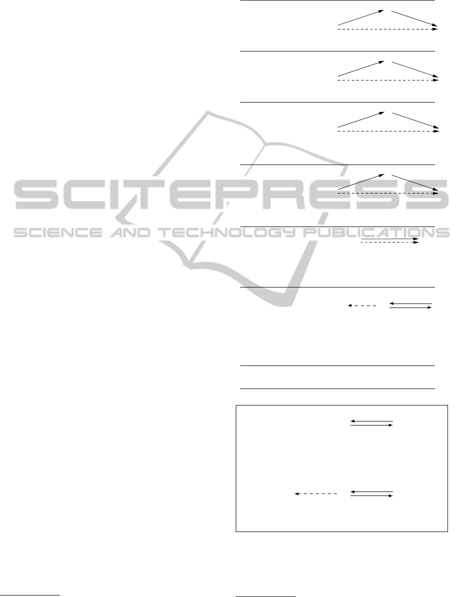
Table 1: Edge-generation rules for the MM5 algorithm. For
each rule, the edge generated by the rule is dashed.
No Case:
S
T
Q
v
u
u + v
Upper Case:
S
T
Q
u
R:v
R: u + v
Lower Case:
S
T
Q
s: u
v
u + v
Applicable if: v < 0 or (v = 0 and S 6≡ T )
Cross Case:
S
T
Q
R: v
R: u + v
s: u
Applicable if: R 6≡ S and (v < 0 or (v = 0 and S 6≡ T ))
Label Removal:
S
T
v
R: v
Applicable if: v ≥ −x, where x is the lower
bound for the contingent link from T to R
serves as a node in the graph;
E
is a set of ordinary
edges;
E
`
is a set of lower-case edges; and
E
u
is a set
of upper-case edges (Morris and Muscettola, 2005).
•
Each ordinary edge has the form,
X
v
Y
, repre-
senting the constraint, Y − X ≤ v.
•
Each lower-case edge has the form,
A
c : x
C
, rep-
resenting the possibility that the contingent dura-
tion, C − A, might take on its minimum value, x.
•
Each upper-case edge,
C
C : −y
A
, represents the
possibility that the contingent duration,
C − A
,
might take on its maximum value, y.
The MM5 algorithm works by recursively gener-
ating new edges in the STNU graph using the rules
shown in Table 1. For each rule, pre-existing edges are
denoted by solid arrows and newly generated edges
are denoted by dashed arrows. Note that each of the
first four rules takes two pre-existing edges as input
and generates a single edge as its output. In contrast,
the Label-Removal rule takes only one edge as input.
Finally, applicability conditions of the form,
R 6≡ S
,
should be construed as stipulating that
R
and
S
must
be distinct time-point variables, not as constraints on
the values of those variables.
Procedure : MM5-DC-Check(G).
Input: G: STNU graph instance to analyze.
Output: the controllability of G.
for 1 to Cutoff Bound do
if (AllMax matrix inconsistent) then
return false;
generate new edges using rules from Table 1;
if (no edges generated) then return true;
end
return false
Note that the edge-generation rules only generate
new ordinary or upper-case edges. Unlike the upper-
case edges in the original graph, the upper-case edges
generated by these rules represent conditional con-
straints, called waits (Morris et al., 2001). In par-
ticular, an upper-case edge,
Y
C : −w
A
, represents a
constraint that as long as the contingent time-point,
C
,
remains unexecuted, then the time-point,
Y
, must wait
at least
w
units after the execution of
A
, the activation
time-point for C.
Procedure : MM5-DC-Check gives pseudocode for
the MM5 DC-checking algorithm. The algorithm per-
forms at most
N
2
+NK +K = O(N
2
)
iterations, which
is the number of distinct kinds of edges in a graph hav-
ing
N
time-points and
K
contingent links. In each iter-
ation, the algorithm first computes the AllMax matrix—
which is the distance matrix for the STN formed by all
of the original and generated, ordinary and upper-case
edges (without their alphabetic labels)—and checks
that there is no negative cycles in it and then applies
the rules from Table 1 to all relevant combinations of
edges of the STNU from the previous iteration. If no
new edges are generated in any given iteration and
there is no negative cycle at all, the algorithm reports
that the network is dynamically controllable. If the al-
gorithm continues generating new, stronger edges after
the cutoff bound
N
2
+ NK + K
, then the network can-
not be DC. Since each iteration can be done in
O(N
3
)
time, the overall complexity of the MM5 algorithm is
O(N
5
).
3.2 CSTNUs
A Conditional Simple Temporal Network with Un-
certainty (CSTNU) is a network that combines the
observation nodes and branching from a CTP with the
contingent links of an STNU (Hunsberger et al., 2012).
There is a one-to-one correspondence between obser-
vation nodes and propositional letters: the execution
of an observation node generates a truth value for the
corresponding proposition. However, nodes and edges
in a CSTNU graph may be labeled by conjunctions of
propositional literals. The time-point corresponding to
AnAlgorithmforCheckingtheDynamicControllabilityofaConditionalSimpleTemporalNetworkwithUncertainty
147

a node with label,
`
, need only be executed in scenarios
where
`
is true. Similarly, the constraint corresponding
to an edge with label,
`
, is only applicable in scenarios
where
`
is true. The label universe, defined below, is
the set of all possible labels.
Definition 1
(Label, Label Universe)
.
Given a set
P
of propositional letters, a label is any (possibly empty)
conjunction of (positive or negative) literals from
P
.
For convenience, the empty label is denoted by
. The
label universe of
P
, denoted by
P
∗
, is the set of all
labels whose literals are drawn from P.
In the following, when not specified, lower-case
Latin letters will denote propositions of
P
, while Greek
lower-case letters will denote labels of P
∗
.
Definition 2 (Consistent labels, label subsumption).
•
Labels,
`
1
and
`
2
, are called consistent, denoted by
Con(`
1
,`
2
), if and only if `
1
∧ `
2
is satisfiable.
•
A label
`
1
subsumes a label
`
2
, denoted by
Sub(`
1
,`
2
), if and only if |= (`
1
⇒ `
2
).
The following definition of a CSTNU is extracted
from Hunsberger et al. (2012). The most important
ingredients of a CSTNU are:
T
, a set of time-points;
C
, a set of labeled constraints;
OT
, a set of observation
time-points; and L a set of contingent links.
Definition 3
(CSTNU)
.
A Conditional STN with Un-
certainty (CSTNU) is a tuple,
hT , C , L, OT , O, P,Li
,
where:
• T is a finite set of real-valued time-points;
• P is a finite set of propositional letters;
• L : T → P
∗
is a function that assigns a label to
each time-point in T ;
• OT ⊆ T is a set of observation time-points;
• O : P → OT
is a bijection that associates a unique
observation time-point to each propositional letter;
• L is a set of contingent links;
• C
is a set of labeled simple temporal constraints,
each having the form,
(Y − X ≤ δ, `)
, where
X,Y ∈ T , δ is a real number, and ` ∈ P
∗
;
•
for any
(Y −X ≤ δ, `) ∈ C
, the label
`
is satisfiable
and subsumes both L(X) and L(Y );
•
for any
p ∈ P
and
T ∈ T
, if
p
or
¬p
appears in
T
’s
label, then
– Sub(L(T ), L(O(p)), and
– (O(p) − T ≤ −ε, L(T )) ∈ C , for some ε > 0;
•
for each
(Y − X ≤ δ, `) ∈ C
and each
p ∈ P
, if
p
or ¬p appears in `, then Sub(`, L(O(p))); and
• (T , bC c, L )
is an STNU, where
bC c
is the follow-
ing set of unlabeled constraints:
{(Y − X ≤ δ) | (Y − X ≤ δ, `) ∈ C for some `}.
The graph for a CSTNU is similar to that for an
STNU except that some of the nodes may be obser-
vation nodes; and there may be propositional labels
on nodes and edges. If
p
is a proposition, then the
observation node whose execution generates a truth
value for
p
shall be denoted by
P?
The propositional
label of a node is usually represented near the node
name, enclosed in square brackets. For example, a
node labeled by
[cd]
is only applicable to scenarios
where propositions
c
and
d
are both true. Since edges
in a CSTNU graph can have both propositional labels
(associated with observation nodes) and alphabetic la-
bels (associated with lower-case and upper-case edges
in an STNU), these different kinds of labels are clearly
distinguished in the labeled values for an edge, as
follows.
Definition 4
(Labeled values)
.
A labeled value is a
triple, hPLabel, ALabel, Numi, where:
• PLabel ∈ P
∗
is a propositional label,
• ALabel
, an alphabetic label, is one of the follow-
ing:
–
an upper-case letter,
C
, as on an upper-case edge
in an STNU;
–
a lower-case letter,
c
, as on a lower-case edge in
an STNU; or
–
, representing no alphabetic label, as for an
ordinary STN edge.
• Num is a real number.
For example,
hp¬q, c, 3i
is a labeled lower-case
edge;
hpq¬r, C, −8i
is a labeled upper-case edge;
and h¬p, , 2i is a labeled ordinary edge.
Fig. 2 shows a sample CSTNU that represents a
possible mapping of the main part of the workflow
schema of Fig. 1. Initially, each ordinary edge in
the network has only one labeled value, while each
edge associated with a contingent link has two labeled
values: one representing an ordinary STN constraint
and the other representing an upper-case or lower-case
STNU constraint. However, the new edge-generation
rules given below will typically result in situations
where a single edge may have numerous labeled val-
ues associated with it. The graph in the figure in-
cludes two observation nodes and three contingent
links. Observation node
A?
generates a truth value for
the proposition,
a
, which represents that the patient in
question is over age 70. Observation node
B?
generates
a truth value for the proposition,
b
, which represents
that the patient is in need of immediate medical atten-
tion. The contingent link,
(C,10, 20, D)
, represents an
Elder Emergency Intervention task that takes between
10 and 20 minutes; the contingent link,
(H, 4, 5, I)
, rep-
resents a Standard Treatment task that takes between
4 and 5 minutes; and the contingent link,
(E, 8, 10, F)
,
ICAART2013-InternationalConferenceonAgentsandArtificialIntelligence
148

B?[]
A?[]
H[¬b]
C[ab]
E[¬ab]
D[ab]
I[¬b]
F[¬ab]
h,, 11ih,, −2i
hab,, 30i
hab,, −16i
h¬ab,, 22i
h¬ab,, −20i
hab,, 5i
hab,, −5i
h¬ab,, 4i
h¬ab,, −2i
h¬b,, 10ih¬b,, −1i
hab,d, 10i
hab,D, −20i
h¬b,i, 4ih¬b,I, −5i
h¬ab, f , 8i
h¬ab,F, −10i
Figure 2: A possible CSTNU graph mapping the main part of the workflow schema of Fig. 1.
represents an Emergency Intervention task that takes
between 8 and 10 minutes. To simplify the graph, only
the lower-case and upper-case edges for each contin-
gent link are explicitly represented.
3
All other edges in
the sample CSTNU represent ordinary temporal con-
straints. For example, the edges between
B?
and
A?
represent that the observation of proposition
a
must
occur between 2 and 11 minutes after the observation
of proposition b.
As defined in Hunsberger et al. (2012), a scenario
s
is a label that specifies a truth value for every propo-
sitional letter. The STNU formed by the nodes and
edges (i.e., time-points and constraints) whose labels
are true in a given scenario is called a projection of the
CSTNU onto that scenario. A situation
ω
for an STNU
specifies fixed durations for all of the contingent links.
A drama
(s,ω)
is a scenario/situation pair that speci-
fies fixed truth values for all of the propositional letters
and fixed durations for all of the contingent links.
An execution strategy is a mapping from dramas
to schedules. A schedule assigns an execution time
to all of the time-points. Thus, if
σ
is an execution
strategy and
(s,ω)
is drama, then
σ(s,ω)
is a schedule.
For any time-point
X
,
[σ(s,ω)]
X
denotes the execution
time assigned to
X
by the strategy
σ
in the drama
(s,ω)
. A dynamic execution strategy is one in which
the execution times assigned to non-contingent time-
points only depends on past observations. A CSTNU is
dynamically controllable if it has a dynamic execution
strategy that guarantees the satisfaction of all temporal
constraints no matter which drama unfolds in real time.
Note that a constraint whose propositional label is
`
need only be satisfied in scenarios where
`
is true.
3
As proven elsewhere (Hunsberger, 2013), the ordinary
edges associated with contingent links are not needed for the
purposes of DC checking.
Similarly, a constraint whose alphabetic label is
C
need
only be satisfied while C remains unexecuted.
Each of the STNUs obtained by projecting the sam-
ple CSTNU of Fig. 2 onto the scenarios,
ab,¬ab
and
¬b
, is dynamically controllable—as an STNU. How-
ever, as will be shown below, the sample CSTNU
is not dynamically controllable—as a CSTNU. This
conforms to the observation by Combi and Posenato
(2010) that the independent controllability of each path
through a workflow is a necessary, but insufficient con-
dition for the controllability of the entire workflow.
For the workflow in Fig. 1, it turns out that there is no
execution time for the observation node,
A?
, that will
enable the rest of the network to be safely executed no
matter how subsequent observations turn out.
4 DC-Checking FOR CSTNUs
This section presents a DC-checking algorithm for
CSTNUs. The basic approach is to extend the MM5
algorithm for STNUs to accommodate propositional
labels. The presence of observation nodes also requires
some new label-modification rules. In addition, since
the propagation of labeled values involves conjoining
labels, which can lead to an exponential number of la-
beled values, the paper also addresses the management
of sets of labeled values.
A partial scenario is a scenario that assigns truth
values to some subset of propositional letters. Partial
scenarios represent the outcomes of past observations.
A label
`
(on a node or edge) is said to be enabled in
a (possibly partial) scenario
s
if none of the proposi-
tional literals in
`
is false in
s
. For example, the label
a¬c
is enabled in the partial scenario
b¬c
, but not in
the partial scenario
bcd
. Note that the truth value of
a
is not determined in either of these partial scenarios.
AnAlgorithmforCheckingtheDynamicControllabilityofaConditionalSimpleTemporalNetworkwithUncertainty
149
During execution of a CSTNU instance, the WfMS
keeps track of all past observations, which together de-
termine a partial scenario. For any as-yet-unexecuted
non-contingent time-point, the WfMS must consider
all enabled labeled constraints involving that time-
point/node and verify that those constraints are sat-
isfiable. For any pair of time-points,
X
and
Y
, it is
possible that more than one labeled constraint from
X
to
Y
is enabled because they are compatible with
the current partial scenario and, therefore, all of them
have to be satisfiable. Thus, it is necessary to generate
all possible constraints/edges for all possible (partial)
scenarios in order to evaluate if a CSTNU is DC con-
trollable. Hereinafter, we indifferently refer to the set
of labeled constraints/edges for a given pair of time-
points as a set of different labeled constraints/edges or
as different labeled values of the same constraint/edge.
4.1 Edge Generation for CSTNUs
The edge generation rules for CSTNUs fall into two
main groups. The first group extends the edge-
generation rules of the MM5 algorithm to accommo-
date labeled edges; the second group consists of label-
modification rules that address interactions involving
observation nodes.
4.1.1 Labeled Constraint Generation
We begin by modifying the edge-generation rules for
STNUs (cf. Table 1) to accommodate labeled edges.
The new rules are shown in Table 2. Note that each of
the first four rules generates an edge whose PLabel is
the conjunction of the PLabels of its parent edges. If
the resulting PLabel is unsatisfiable (e.g.,
p¬p
), then
the new edge is not generated (or kept). The fifth rule
effectively removes the upper-case (alphabetic) label,
resulting in a labeled ordinary edge.
The sixth rule, the Observation Case rule, does not
extend any of the MM5 rules; however, it is included
here for convenience. This new rule addresses circum-
stances where an existing labeled edge from
X
to
Y
is
inconsistent with an existing labeled edge from
Y
to
X
.
To avoid having to satisfy both of these constraints—
which would be impossible—this rule adds a new edge
that ensures that the value of the proposition
p
, which
appears in both labels, will be known before having to
decide which constraint to satisfy. The soundness of
this rule is ensured by the following lemma.
Lemma 4.1
(Observation Case)
.
Let
σ
be a dynamic
execution strategy that satisfies the labeled constraints
in Fig. 3-(a). Then
σ
must also satisfy the labeled
constraint, (P? −Y ≤ 0, αβγ), shown in Fig. 3-(b).
4
4
Recall that an execution strategy need only satisfy la-
Table 2: New edge-generation rules for CSTNUs.
Labeled No Case:
S
T
Q
hα, , ui
hβ, , vi
hαβ, , u + vi
Labeled Upper Case:
S
T
Q
hα, , ui
hβ, R, vi
hαβ, R, u + vi
Labeled Lower Case:
S
T
Q
hα, s, ui
hβ, , vi
hαβ, , u + vi
Applicable if: v < 0 or (v = 0 and S 6≡ T )
Labeled Cross Case:
S
T
Q
hα, s, ui
hβ, R, vi
hαβ, R, u + vi
Applicable if: R 6≡ S and (v < 0 or (v = 0 and S 6≡ T ))
Labeled Label Removal:
S
T
hα, R, vi
hα, , vi
Applicable if: v ≥ −x, where x is the lower
bound for the contingent link from T to R
Observation Case:
P?
Y X
hαβγ,,0i
hαβp, ,ui
hβγ¬p,,−vi
Applicable if: 0 ≤ u < v, and α,β and γ are labels
that do not share any literals; and p,¬p are literals
that do not appear in α, β or γ.
Note: Only new edges with satisfiable labels are kept.
P?
Y X
hαβp, ,ui
hβγ¬p,,−vi
(a)
Pre-existing edges, where
0 ≤ u < v
, and
α,β
and
γ
are labels that do not share any literals; and
p,¬p
are literals that do not appear in α,β or γ.
P?
Y X
hαβγ,,0i
hαβp, ,ui
hβγ¬p,,−vi
(b) Generated edge (dashed).
Figure 3: The Observation Case Rule (cf. Lemma 4.1).
Proof.
Let
σ
be as in the statement of the lemma. Sup-
pose there is a drama, (s,ω), such that:
beled constraints in scenarios where their labels are true.
ICAART2013-InternationalConferenceonAgentsandArtificialIntelligence
150

• the label αβγ is true in scenario s; but
•
the schedule
σ(s,ω)
does not satisfy the constraint,
(P? −Y ≤ 0, αβγ).
Then, in that schedule,
P? −Y > 0
and, hence,
Y < P?
Next, since
X −Y ≤ −v < 0,
it follows that
X < Y
.
Thus, X < Y < P? (i.e., both X and Y precede P?).
Next, let
˜s
be the same scenario as
s
except that
the truth value of
p
is flipped. Let
t
be the first time at
which the schedules,
σ(s,ω)
and
σ( ˜s, ω)
, differ. Thus,
there must be some time-point
T
that is executed in
one of the schedules at time
t
, and in the other at some
time later than
t
. In that case, the corresponding histo-
ries (of past observations) at time
t
must be different.
However, since all other propositions and contingent
durations are identical in the dramas,
(s,ω)
and
( ˜s, ω)
,
the only possible difference must involve the value of
the proposition
p
, whence
P?
must be executed in both
schedules before the time of first difference, t.
Now, in the schedule
σ(s,ω)
, we have seen that
both
X
and
Y
are executed before
P?
, and hence be-
fore
t
. Thus,
[σ(s,ω)]
X
= [σ( ˜s, ω)]
X
and
[σ(s,ω)]
Y
=
[σ( ˜s, ω)]
Y
. But this is not possible because in one sce-
nario
Y − X ≤ u
, while in the other
Y − X ≥ v
. In
particular, both constraints cannot be satisfied, using
the same values of X and Y , since u < v.
4.1.2 Label Modification
This section introduces a variety of label-modification
rules that share some resemblance to the Label-
Removal rule in Table 2. Thus, we begin with a short
description of the Label-Removal rule.
Suppose a CSTNU contains a contingent link,
(A,5,12,C)
. In other words, the contingent duration,
C − A
, is uncontrollable, but guaranteed to be within
the interval,
[5,12]
. Suppose further that the network
also contains the upper-case edge,
Y
C : −2
A
, which
represents the following wait constraint: “As long as
the contingent time-point
C
remains unexecuted, then
Y
must wait at least
2
units after the execution of its ac-
tivation time-point,
A
.” Given that the minimum dura-
tion of this contingent link is
5
, it follows that the con-
tingent time-point
C
must remain unexecuted until af-
ter the wait time of
2
has expired. As a result, the deci-
sion to execute
Y
must, in every situation, wait at least
2
units after
A
. For this reason, the Label-Removal
rule generates the ordinary edge,
Y
−2
A
, which rep-
resents the unconditional constraint,
A −Y ≤ −2
(i.e.,
Y ≥ A + 2
). This example illustrates that in certain cir-
cumstances, a constraint conditioned on an uncontrol-
lable event—in this case, the execution of the contin-
gent time-point
C
—might have the force of an uncon-
ditional constraint because the uncertainty associated
Table 3: Label-modification rules for CSTNUs. Labeled
values in shaded boxes replace those in dashed boxes.
R0 Case:
P?
X
hαp, ~,−wi
hα,~,−wi
Applicable if:
0 ≤ w
,
p
is a literal not in
α
, and
~
is
either or an upper-case letter.
R1 Case:
P?
X Y
hαβ,,−wi hβγp, ~,vi
hαβγ,~,vi
h¬αβγp,~,vi
Applicable if:
0 ≤ w
;
v ≤ w
;
α,β
and
γ
are labels that
do not share any literals;
p
is a literal that does not
appear in α,β or γ; and ~ is or an upper-case letter.
R2 Case:
P?
X
hαβ,,−wi
hβγp, ~,vi
hαβγ,~,vi
h¬αβγp,~,vi
Applicable if:
0 ≤ w ≤ v
;
α,β
and
γ
are labels that do
not share any literals;
p
is a literal that does not appear
in α,β or γ; and ~ is either or an upper-case letter.
R3 Case:
P?
X Y
hαβ,,−wi hβγp, ~,−vi
hαβγ,~,−vi
h¬αβγp,~,−vi
Applicable if:
0 ≤ w
;
v ≤ w
;
α,β
and
γ
are labels that
do not share any literals;
p
is a literal that does not
appear in α,β or γ; and ~ is or an upper-case letter.
with the uncontrollable event will definitely not be re-
solved at the time a particular execution decision—in
this case, the decision to execute Y —must be made.
The label-modification rules in Table 3 have the
same general flavor, except that they deal with the
uncertainty associated with observation nodes, rather
than contingent links. For example, consider the edge,
P?
hαp, , −wi
X
, where neither
p
nor
¬p
appears
in
α
, and
w ≥ 0
. This edge represents the condi-
tional constraint that “in scenarios where
αp
is true,
X −P? ≤ −w
(i.e.,
X +w ≤ P?)
must hold.” Given
that
w ≥ 0
, it follows that in scenarios where
αp
is
true,
X
must be executed before the observation node
P?
But that, in turn, implies that the truth value of
p
cannot be known at the time
X
is executed. And, of
course, the truth value of
p
cannot be known when the
decision to execute
P?
is made either. As a result, deci-
sions about when to execute
X
and
P?
cannot depend
on the truth value of
p
. Thus, the PLabel on the edge
from
P?
to
X
should be modified to remove the occur-
rence of
p
, yielding the new edge,
P?
hα, , −wi
X
,
which represents the constraint that in scenarios where
α
holds,
X − P? ≤ −w
(i.e.,
X + w ≤ P?
) must hold.
AnAlgorithmforCheckingtheDynamicControllabilityofaConditionalSimpleTemporalNetworkwithUncertainty
151
This is the idea behind the label-modification rule,
R0, shown in Table 3. For each rule in the table, pre-
existing labels are represented as usual, labels to be
modified (or replaced by new ones) are shown within
a dashed box, and newly generated labels are shown
within a shaded box. The following lemma shows that
Rule R0 is sound.
P?
X
hαp, ~,−wi
(a)
Pre-existing edge, where
0 ≤ w
,
p
is a literal that
does not appear in
α
, and
~
can be either
or an
upper-case letter.
P?
X
hα,~,−wi
(b) Modified label.
Figure 4: The Label-Modification rule, R0 (cf. Lemma 4.2).
Lemma 4.2
(Label-Modification Rule, R0)
.
Suppose
that
w ≥ 0
and
α
is a label that does not contain the
literal
p
. If
σ
is a dynamic execution strategy that
satisfies the labeled constraint,
(X −P? ≤ −w,αp)
, as
shown in Fig. 4-(a), then
σ
must also satisfy the labeled
constraint,
(X − P? ≤ −w, α)
, as shown in Fig. 4-(b).
The rule also applies to upper-case edges (i.e., edges
with an upper-case alphabetic label, ~).
Proof. Let (s, ω) be a drama such that:
• the label α¬p is true in scenario s; but
•
the schedule
σ(s,ω)
does not satisfy the constraint,
(X −P? ≤ −w).
In that case,
X + w > P?
Next, let
s
0
be the same
scenario as
s
except that
p
is true in
s
0
. Then
αp
is
true in
s
0
, which implies that
(X −P? ≤ −w)
holds in
σ(s
0
,ω). Thus, X + w ≤ P? holds in σ(s
0
,ω).
Next, let
t
be the first time at which the schedules,
σ(s,ω)
and
σ(s
0
,ω)
, differ. Then there must be some
time-point
T
that is executed in one of the schedules
at time
t
, and in the other at some time after
t
. But in
that case, the corresponding histories at time
t
must
be different. Since the dramas,
(s,ω)
and
(s
0
,ω)
, are
identical except for the truth value of
p
, it follows
that the observation node,
P?
, must be executed be-
fore time
t
. Now, in the drama
(s
0
,ω)
, the constraint,
X + w ≤ P?
, is satisfied; thus, both
X
and
P?
must
be executed before time
t
in that drama. Since the
schedules,
σ(s,ω)
and
σ(s
0
,ω)
, are identical prior to
time
t
, it follows that the same constraint is satisfied
by σ(s
0
,ω), contradicting the choice of (s
0
,ω).
Rule R1 in Table 3 first appeared in Hunsberger
et al. (2012). The corresponding lemma, given below,
shows that it is sound. Its proof is not repeated here.
Lemma 4.3
(Label-Modification Rule, R1)
.
Let
σ
be
a dynamic execution strategy that satisfies the labeled
constraints in Fig. 5-(a). Then
σ
must also satisfy
the labeled constraint
(Y − X ≤ v, αβγ)
. The original
constraint,
(Y − X ≤ v,βγp)
, is replaced by the pair
of labeled constraints,
(Y − X ≤ v, αβγ)
and
(Y − X ≤
v,¬αβγp), as depicted in Fig. 5-(b).
P?
X
Y
hαβ,,−wi hβγp, ~,vi
(a)
Pre-existing edges, where
0 ≤ w, v ≤ w
;
α,β
and
γ
are labels that do not share any literals;
p
is a literal
that does not appear in
α,β
or
γ
; and
~
is either
or an upper-case letter.
P?
X Y
hαβ,,−wi
hαβγ,~,vi
h¬αβγp,~,vi
(b) New labels on the edge from X to Y .
Figure 5: The Label-Modification rule, R1 (cf. Lemma 4.3).
Regarding the proof, here we only remark that
when
v > w
the rule is not needed because, in that
case, the execution of
Y
could be postponed until after
the execution of
P?
, in which case the truth value of
p
would become known.
Lemma 4.3 does not analyze the case where
P?
and
Y
are the same node. In that case, rule R1 is
not needed. In particular, if
v < w
, there would be a
negative cycle, implying that the network was not DC.
However, we need to consider the case where
P?
and
Y
are the same node and
v ≥ w
. In that case, the label
βγp
must always be considered before the execution
of
P?
(i.e., before the truth value of
p
is known) and,
therefore, it is necessary to propagate it without
p
. We
call this rule R2.
Lemma 4.4
(Label-Removal Rule, R2)
.
Let
σ
be a
dynamic execution strategy that satisfies the labeled
constraints in Fig. 6-(a). Then
σ
must also satisfy
the labeled constraint,
(Y − X ≤ v,αβγ)
. The original
constraint,
(Y − X ≤ v,βγp)
, is replaced by the pair
of labeled constraints,
(Y − X ≤ v, αβγ)
and
(Y − X ≤
v,¬αβγp), as depicted in Fig. 6-(b).
Proof.
It is straightforward to prove the soundness of
this rule, since it deals with the standard constraint
between two ordered time-points.
When there is a negative value on a constraint from
Y
to
X
, we have another case of label modification as
shown in the following lemma.
Lemma 4.5
(Label-Modification Rule, R3)
.
Let
σ
be
a dynamic execution strategy that satisfies the labeled
ICAART2013-InternationalConferenceonAgentsandArtificialIntelligence
152

P?
X
hαβ,,−wi
hβγp, ~,vi
(a)
Pre-existing edges, where
0 ≤ w, v ≥ w
;
α,β
and
γ
are labels that do not share any literals;
p
is a literal
that does not appear in
α,β
or
γ
; and
~
is either
or an upper-case letter.
P?
X
hαβ,,−wi
hαβγ,~,vi
h¬αβγp,~,vi
(b) New labels on the edge from Y to X.
Figure 6: The Label-Modification rule, R2 (cf. Lemma 4.4).
constraints shown in Fig. 7-(a). Then
σ
must also
satisfy the labeled constraint,
(X −Y ≤ −v,αβγ)
. The
original constraint,
(X −Y ≤ −v,βγp)
, is replaced by
the pair of labeled constraints,
(X −Y ≤ −v, αβγ)
and
(X −Y ≤ −v,¬αβγp), as shown in Fig. 7-(b).
P?
X Y
hαβ,,−wi hβγp, ~,−vi
(a)
Pre-existing edges, where
0 ≤ w
;
v ≤ w
;
α,β
and
γ
are labels that do not share any literals;
p
is a literal
that does not appear in
α,β
or
γ
; and
~
is either
or an upper-case letter.
P?
X Y
hαβ,,−wi
hαβγ,~,−vi
h¬αβγp,~,−vi
(b) New labels on the edge from Y to X.
Figure 7: The Label-Modification rule, R3 (cf. Lemma 4.5).
Proof.
Let
σ
be as in the statement of the lemma. Sup-
pose that there is some drama, (s,ω), such that:
• the label αβγ is true in scenario s; but
•
the schedule
σ(s,ω)
, does not satisfy the con-
straint, (X −Y ≤ −v).
In that case,
X −Y > −v,
which implies that
Y < X + v ≤ X + w ≤ P?
(Recall that
v ≤ w
and,
given that
αβ
is true, the constraint,
(X −P? ≤ −w),
must be satisfied by σ.) Note also that X ≤ P?
Next, let
˜s
be the same scenario as
s
except that
the truth value of
p
is flipped. Let
t
be the first time
at which the schedules,
σ(s,ω)
and
σ( ˜s, ω)
, differ.
Thus, there must be some time-point
T
that is exe-
cuted in one of the schedules at time
t
, and in the
other at some time later than
t
. But in that case,
the corresponding histories at time
t
must be differ-
ent. But the only possible difference must involve
the value of the proposition
P?
, since all other propo-
sitions and contingent durations are identical in the
dramas,
(s,ω)
and
( ˜s, ω)
. Thus,
P?
must be executed
before time
t
. Now, in the schedule
σ(s,ω)
, we have
seen that both
Y
and
X
are executed before
P?
, and
hence before
t
. Thus,
[σ(s,ω)]
X
= [σ( ˜s, ω)]
X
and
[σ(s,ω)]
Y
= [σ( ˜s, ω)]
Y
. But then the value of
Y − X
must be the same in both schedules. Thus, the con-
straint
X −Y ≤ −v
must be violated in both schedules.
But this contradicts that the constraint
X −Y ≤ −v
is
satisfied in scenarios where βγp is true.
Regarding the constraint
(X −Y ≤ −v, ¬αβγp)
, it
is straightforward to show that it is necessary to in-
troduce it to maintain equivalence with the original
constraint from
Y
to
X
.
5
Indeed, when
α
is false, the
relation between P? and X is not known.
The application of rules R0, R1, R2 and R3 has to
be considered for all pairs of time-points with respect
to all suitable observation points.
4.2 A CSTNU DC-Checking Algorithm
This section presents an algorithm for determining
whether arbitrary CSTNU instances are dynamically
controllable.
This DC-checking algorithm works by applying
the labeled constraint-generation rules of Table 2 and
the label-modification rules of Table 3 to all relevant
combinations of edges until:
•
the associated AllMax matrix is found to be incon-
sistent; or
•
the rules cannot generate any more new (stronger)
edges; or
•
a maximum number of rounds of rule applications
has been reached.
The pseudocode for the algorithm is shown in Proce-
dure : CSTNU-DC-Check, below.
The algorithm performs
p(n
2
+ nk + k)
rounds,
where
n
is the number of time-points,
k
is the number
of contingent links, and
p
is the number of proposi-
tional letters that appear in the network. In each round,
all of the label-modification rules from Table 3 are first
applied, followed by the edge-generation rules from
Table 2. After those rounds have completed, if it is
still possible to generate stronger constraints having
the same labels, then the CSTNU is not DC. Proof of
this is an easy extension of Morris and Muscettola’s
argument about the number of rounds in the MM5
algorithm.
Given the lemmas presented in this paper, it is
straightforward to verify that the algorithm is sound.
5
A similar check is done by Hunsberger et al. (2012).
AnAlgorithmforCheckingtheDynamicControllabilityofaConditionalSimpleTemporalNetworkwithUncertainty
153

Procedure : CSTNU-DC-Check(G).
Input: G =
hT , C ,L,OT , O, P, Li: a CSTNU instance
Output: the dynamic controllability of G.
G
0
= G;
for 1 to |P|(|T |
2
+ |T ||L| + |L|) do
if (AllMax matrix of G is inconsistent) then
return false;
// Label Modification Rules
G =LabelModificationRuleR0(G);
G =LabelModificationRuleR1(G);
G =LabelModificationRuleR2(G);
G =LabelModificationRuleR3(G);
// Labeled Constraints Generation
G
0
= G
0
∪ needed LabeledNoCaseRule(G);
G
0
= G
0
∪ needed LabeledUpperCaseRule(G);
G
0
= G
0
∪ any LabeledCrossCaseRule(G);
G
0
= G
0
∪ any LabeledLowerCaseRule(G);
G
0
= G
0
∪ any LabeledLabelRemovalRule(G);
G
0
= G
0
∪ any ObservationCaseRule(G);
if (no rules were applied) then return true;
G = G
0
;
return false
Thus, whenever the algorithm is given a DC network,
the algorithm invariably declares it to be DC. Stated
differently, the algorithm never generates false nega-
tives (i.e., if the algorithm declares a network to be
non-DC, then the network must be non-DC).
We are continuing to study the question of com-
pleteness. (A DC-checking algorithm is complete if it
never generates false positives—that is, it only says a
network is DC if it really is DC.)
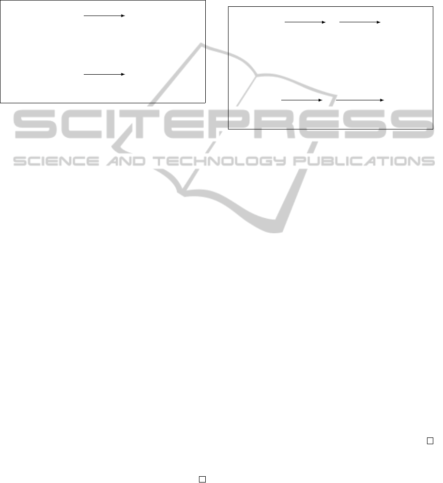
4.2.1 On the Management of PropLabels
The actual performance of the algorithm can also be af-
fected by the strategy for managing the sets of labeled
values on edges in the graph. To better introduce the
issue, let us consider the application of the No-Case
rule to a pair of constraints containing different la-
beled values, as in the example of Fig. 8. Even though,
for a given edge, only the minimal value is stored
for each possible label, it is still possible to have an
exponential explosion in the number of labeled val-
ues, as suggested by Fig. 8-(a). However, exponential
numbers of labeled values are not always necessary
because it is possible that some subsets of labeled val-
ues might be represented by just one. For example, the
pair of labeled values,
h¬A,,10i
and
hA,,10i
, can
be represented by the single labeled value,
h,,10i
.
In addition, since this labeled value is stronger than
the labeled value,
h,,12i
, the latter labeled value
is redundant. Similar reasoning shows that the six
labeled values on the edge from
Q
to
T
in Fig. 8-(a)
can be replaced by the two labeled values shown in
Q
S
T
h,,6i, h¬A,, 4i
h¬B,,4i
h,,6i, hA,, 4i
h¬B,,4i
h,,12i, hA,, 10i,
h¬A,,10i, h¬A¬B, , 8i
hA¬B,,8i, h¬B, , 8i
(a): Without management of labeled values.
Q
S
T
h,,6i, h¬A,, 4i
h¬B,,4i
h,,6i, hA,, 4i
h¬B,,4i
h,,10i, h¬B,, 8i
(b): Optimal management of labeled values.
Figure 8: Two different strategies for managing the storage
of labeled values in an application of the No-Case rule.
Fig. 8-(b). In the following we propose some labeled-
value-management rules with the aim of minimizing
the number of labeled values stored with each edge.
When there are two or more labeled values with
labels that subsume the same “seed” label, and they
have all the same numerical value, it is not necessary to
explicitly represent all of them. Instead, it is sufficient
to represent only the “seed” one. For example, the two
labeled values of Fig. 8,
hA¬B,,8i
and
h¬B,,8i
can
be replaced by the single labeled value, h¬B, , 8i.
Rule 1
(Redundant Label Elimination 1, RLE 1)
.
If
a set of labeled values contains two labels
(`
1
,i)
and
(`
2
,i)
where
`
1
subsumes
`
2
, then the labeled value
(`
1
,i) is redundant and it can be removed.
The previous rule can be simply extended to the
case when two labels differ for only one proposition.
Rule 2
(Redundant Label Elimination 2, RLE 2)
.
If
a set of labeled values contains two labeled values,
(αp, i)
and
(α¬p, j)
, where
α
contains neither
p
nor
¬p, there are two cases:
1.
if
i = j
, then both labeled values can be represented
by (α,i).
2.
if
i 6= j
, then remove any labeled values of the form,
(α,k)
, since the value of
k
would be greater than
both i and j, making the labeled value redundant.
For example, in Fig. 8,
hA¬B,,8i
and
h¬A¬B,,8i can be replaced by h¬B, , 8i.
Regarding the empty label (
), it effectively rep-
resents the disjunction of all possible labels. Thus,
if there is an empty-labeled value, that value can be
considered to be the default value. If there are other
labeled values, their numerical values must be smaller
than the numerical values associated with the default;
otherwise, RLE 1 applies. It is possible to represent all
possible combinations of labels not only with an empty
ICAART2013-InternationalConferenceonAgentsandArtificialIntelligence
154

label, but also with a suitable set of labels. For exam-
ple, in the set
{hA,,8i,h¬A,,8i,h,,10i}
, the pair
of labels
hA,,8i
and
h¬A,,8i
represent all possible
labels of the Universe and their values are smaller than
the empty-labeled one. Thus, the empty labeled value
can be removed. These observations lead to rule RLE3,
below.
Rule 3
(Empty Label Elimination, RLE 3)
.
If a set of
labeled values contains a subset of labels that cover all
possible combinations of a fixed set of propositions,
then such a subset represents the base of all possible
labels. Therefore, any empty-labeled value can be
removed since, by construction, its numerical value
must be greater than the numerical values associated
with the labels of the base.
These rules explain how to maintain a set of labeled
values for a given edge in order to rightly represent
all the possible values, while maintaining the minimal
number of such values represented explicitly.
In general, if we have to add the labeled values
of a set
S
1
to the labeled values of a set
S
2
(e.g.,
as must be done when applying the No-Case rule
to a pair of labeled edges), it is necessary to add
each labeled value of the first set to each each la-
beled value of the second set.
6
The propositional
label for the sum of the two labeled values is the
conjunction of the two involved propositional labels.
Assuming that those propositional labels are consis-
tent, the new labeled value is put into a new set that
represents the result of the overall operation. For ex-
ample, given the two sets of labeled values seen in
Fig. 8-(a),
S
1
= {h, , 6i, h¬A, , 4i, h¬B, , 4i}
and
S
2
= {h, , 6i, hA, , 4i, h¬B, , 4i}, their sum is:
S
1
+ S
2
= {h, , 6i + h, , 6i = h, , 12i, (1)
h,,6i + hA,,4i = hA, , 10i, (2)
h,,6i + h¬B,,4i = h¬B, , 10i, (3)
h¬A,,4i + h,,6i = h¬A, , 10i, (4)
h¬A,,4i + hA,,4i = inconsistent, (5)
h¬A,,4i + h¬B,,4i = h¬A¬B, , 8i, (6)
h¬B,,4i + h,,6i = h¬B, , 10i, (7)
h¬B,,4i + hA,,4i = hA¬B, , 8i, (8)
h¬B,,4i + h¬B,,4i = h¬B, , 8i} (9)
The sum of the labeled values in line (5) does not
generate a new labeled value since the propositional
labels,
A
and
¬A
, are inconsistent. The rest of the
newly generated labeled values can be represented by
a small number of labeled values, as determined by
the label-elimination rules. For example,
h¬B,,8i
makes
h¬B,,10i
redundant. Next, rule RLE2 says
6
Similar issues were discussed by Conrad et al. (2011).
that
hA¬B,,8i
and
h¬A¬B,,8i
can be replaced by
h¬B,,8i
, which is already present (Line 9). Finally,
rule RLE1 says that
h¬A,,10i
and
hA,,10i
can be
replaced by
h,,10i
, which dominates the constraint,
h,,12i
, which is present in Line 1. Hence, the
“reduced” set becomes:
S
1
+ S
2
= {h, , 10i, h¬B, , 8i}
5 DISCUSSION
AND CONCLUSIONS
To verify and test the practical usability of the pro-
posed algorithm, we have built a Java program, called
CSTNU EDITOR, that allows one to graphically de-
sign a CSTNU instance and to check its dynamic con-
trollability. Fig. 9 depicts a screen shot of the program
running on a sample CSTNU instance.
The program implements a variety of strategies
for managing the sets of labeled values which enables
the user to better monitor the propagation of labeled
values and its impact on the convergence of the algo-
rithm. Preliminary experiments show that the algo-
rithm finds the solution in an average number of cycles
one order of magnitude smaller than the theoretical
estimated upper bound. Moreover, different policies
in the management of labeled value sets have different
consequences on the convergence of the algorithm: the
number of cycles required to find a solution decreases
when the management strategy minimizes (in any way)
the number of stored labels, but the running time of
each cycle of the algorithm increases. We are currently
evaluating which management strategy provides the
best trade-off between the sizes of the labeled value
sets and execution time.
In summary, this paper presented a DC-checking
algorithm for CSTNUs. The algorithm uses rules for
generating labeled constraints/edges that extend the
rules presented by Morris et al. (2005). It also uses new
label-modification rules needed to manage different
possible alternative executions. It is the first such
algorithm in the literature. The algorithm is proven to
be sound.
As for future work, we are going to formally ana-
lyze whether the algorithm is complete. Moreover, we
will extensively test CSTNU EDITOR with synthetic
and real world complex CSTNU networks in order
to evaluate its applicability in the area of temporal
workflow systems.
AnAlgorithmforCheckingtheDynamicControllabilityofaConditionalSimpleTemporalNetworkwithUncertainty
155
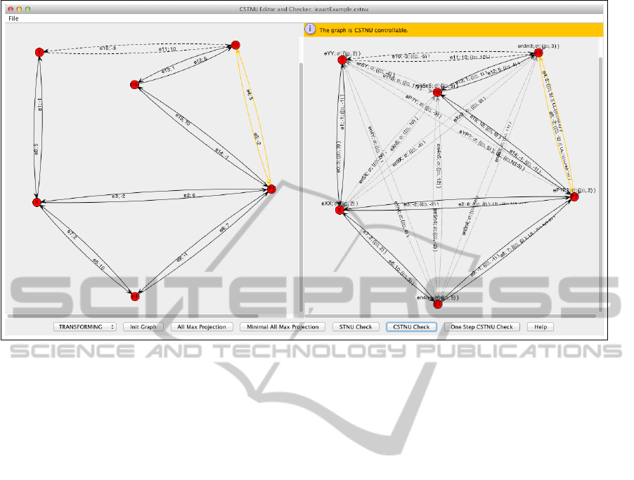
Figure 9: A screen shot of the CSTNU editor and checker.
REFERENCES
Combi, C. and Posenato, R. (2010). Towards temporal con-
trollabilities for workflow schemata. In (Markey and
Wijsen, 2010), pages 129–136.
Conrad, P. R. and Williams, B. C. (2011). Drake: An efficient
executive for temporal plans with choice. Journal of
Artificial Intelligence Research (JAIR), 42:607–659.
Dechter, R., Meiri, I., and Pearl, J. (1991). Temporal con-
straint networks. Artificial Intelligence, 49(1-3):61–95.
Hunsberger, L. (2009). Fixing the semantics for dynamic
controllability and providing a more practical charac-
terization of dynamic execution strategies. In Lutz, C.
and Raskin, J.-F., editors, The 16th International Sym-
posium on Temporal Representation and Reasoning
(TIME-2009), pages 155–162. IEEE.
Hunsberger, L. (2010). A fast incremental algorithm for
managing the execution of dynamically controllable
temporal networks. In (Markey and Wijsen, 2010),
pages 121–128.
Hunsberger, L. (2013). Magic loops in simple temporal
networks with uncertainty. In Fifth International Con-
ference on Agents and Artificial Intelligence (ICAART-
2013). SciTePress.
Hunsberger, L., Posenato, R., and Combi, C. (2012). The
Dynamic Controllability of Conditional STNs with Un-
certainty. In Workshop on Planning and Plan Execu-
tion for Real-World Systems: Principles and Practices
(PlanEx) @ ICAPS-2012, pages 1–8, Atibaia.
Markey, N. and Wijsen, J., editors (2010). The Seventeenth
International Symposium on Temporal Representation
and Reasoning (TIME-2010). IEEE.
Morris, P. (2006). A structural characterization of tempo-
ral dynamic controllability. In Benhamou, F., editor,
Principles and Practice of Constraint Programming,
volume 4204 of LNCS, pages 375–389. Springer.
Morris, P. H. and Muscettola, N. (2005). Temporal dynamic
controllability revisited. In Veloso, M. M. and Kamb-
hampati, S., editors, The Twentieth National Confer-
ence on Artificial Intelligence (AAAI-05), pages 1193–
1198. AAAI Press.
Morris, P. H., Muscettola, N., and Vidal, T. (2001). Dynamic
control of plans with temporal uncertainty. In Nebel, B.,
editor, The Seventeenth International Joint Conference
on Artificial Intelligence (IJCAI-01), pages 494–502.
Morgan Kaufmann.
Tsamardinos, I., Vidal, T., and Pollack, M. E. (2003). CTP:
A new constraint-based formalism for conditional, tem-
poral planning. Constraints, 8:365–388.
ICAART2013-InternationalConferenceonAgentsandArtificialIntelligence
156
