
Magic Loops in Simple Temporal Networks with Uncertainty
Exploiting Structure to Speed Up Dynamic Controllability Checking
Luke Hunsberger
Computer Science Department, Vassar College, Poughkeepsie, NY, U.S.A.
Keywords:
Temporal Networks, Dynamic Controllability.
Abstract:
A Simple Temporal Network with Uncertainty (STNU) is a structure for representing and reasoning about
temporal constraints and uncontrollable-but-bounded temporal intervals called contingent links. An STNU is
dynamically controllable (DC) if there exists a strategy for executing its time-points that guarantees that all
of the constraints will be satisfied no matter how the durations of the contingent links turn out. The fastest
algorithm for checking the dynamic controllability of arbitrary STNUs is based on an analysis of the graphical
structure of STNUs. This paper (1) presents a new method for analyzing the graphical structure of STNUs,
(2) determines an upper bound on the complexity of certain structures—the indivisible semi-reducible negative
loops; (3) presents an algorithm for generating loops—the magic loops—whose complexity attains this upper
bound; and (4) shows how the upper bound can be exploited to speed up the process of DC-checking for certain
networks. Theoretically, the paper deepens our understanding of the structure of STNU graphs. Practically, it
demonstrates new ways of exploiting graphical structure to speed up DC checking.
1 BACKGROUND
Agent-based applications invariably involve actions
and temporal constraints. Dechter et al. (1991) in-
troduced Simple Temporal Networks (STNs) to fa-
cilitate the management of temporal constraints. Vi-
dal and Ghallab (1996) were the first to incorpo-
rate actions with uncertain durations into an STN-
like framework, and to define a notion of dynamic
controllability. Morris et al. (2001) developed the
most widely accepted formalization of Simple Tem-
poral Networks with Uncertainty (STNUs) and dy-
namic controllability. Morris and Muscettola (2005)
developed an O(N
5
)-time algorithm for checking the
dynamic controllability of arbitrary STNUs. Mor-
ris (2006) presented an O(N
4
)-time DC-checking al-
gorithm that was based on an analysis of the structure
of STNU graphs; it is the fastest DC-checking algo-
rithm reported so far in the literature.
⇒ This paper presents a new way of analyzing the
structure of STNU graphs that can be used to
speed up DC checking for some networks.
The rest of this section summarizes the definitions and
results for STNs, STNUs and dynamic controllability
that will be used in the rest of the paper.
1.1 Simple Temporal Networks
Dechter et al. (1991) introduced Simple Temporal
Networks (STNs) and presented the basic theoretical
results for them. An STN is a pair, (T , C), where T is
a set of time-point variables (or time-points) and C is
a set of constraints, each having the form, Y − X ≤ δ,
for some X,Y ∈ T , and real number δ. Typically, the
time-points in T represent starting or ending times
of actions, or abstract coordination times. The con-
straints in C can accommodate release, deadline, du-
ration and inter-action constraints. An STN is consis-
tent if there exists a set of values for its time-points
that together satisfy all of its constraints.
For any STN, S = (T , C), there is a correspond-
ing graph, G, where the nodes in G correspond to the
time-points in T , and for each constraint, Y − X ≤ δ,
in C , there is an edge in G of the form, X
−
→
δ
Y .
For convenience, this paper calls the constraints and
edges in an STN ordinary constraints and edges.
The all-pairs, shortest-paths matrix for G is called
the distance matrix for S (or G) and is denoted by D.
Thus, for any X and Y in T , D(X,Y ) equals the length
of the shortest path from X to Y in the graph G. If D
has nothing but zeros down its main diagonal, then D
is said to be consistent.
Theorem 1 (Fundamental Theorem of STNs). For
157
Hunsberger L..
Magic Loops in Simple Temporal Networks with Uncertainty - Exploiting Structure to Speed Up Dynamic Controllability Checking.
DOI: 10.5220/0004260501570170
In Proceedings of the 5th International Conference on Agents and Artificial Intelligence (ICAART-2013), pages 157-170
ISBN: 978-989-8565-39-6
Copyright
c
2013 SCITEPRESS (Science and Technology Publications, Lda.)

any STN S, with graph G, and distance matrix D,
the following are equivalent:
• S is consistent.
• G has no negative loops.
• D is consistent.
1.2 STNs with Uncertainty
Some applications involve actions whose durations
are uncontrollable, but nonetheless guaranteed to fall
within known bounds. For example, when I turn on
my laptop, I do not control how long it will take to
load its operating system; however, I know that it
will take anywhere from one to four minutes. A Sim-
ple Temporal Network with Uncertainty (STNU) aug-
ments an STN to include contingent links that repre-
sent this kind of uncontrollable-but-bounded tempo-
ral interval (Morris et al., 2001). A contingent link
has the form, (A,x,y,C), where A and C are time-
points and 0 < x < y < ∞. A is called the activation
time-point; C is called the contingent time-point. In-
tuitively, the duration of the interval from A to C is
uncontrollable, but guaranteed to fall within the inter-
val [x,y]. Typically, an agent controls the execution
of the activation time-point A, but only observes the
execution of the contingent time-point C in real time.
1
Thus, an STNU is a triple, (T ,C ,L), where
(T , C) is an STN, and L is a set of contingent links.
N is used to denote the number of time-points in an
STNU, K the number of contingent links.
The most important property of an STNU is
whether it is dynamically controllable (DC)—that is,
whether there exists a strategy for executing the non-
contingent time-points that guarantees that all of the
constraints in the network will be satisfied no mat-
ter how the contingent durations turn out. The strat-
egy is dynamic in that its execution decisions are al-
lowed to depend on and react to past observations,
but not present or future observations. The formal
semantics for dynamic controllability is quite com-
plicated, but it need not be presented here because a
more convenient—and equivalent—graphical charac-
terization is available, as follows.
Graph for an STNU. Let S = (T , C,L) be an
STNU. The graph for S contains all of the edges
from the STN, (T ,C ), as well as additional edges
derived from the contingent links in L. In particu-
lar, for each contingent link (A,x,y,C) ∈ L, the graph
contains the edges shown in Fig. 1. The ordinary
edges, A
−→
y
C and C
−→
−x
A, represent the or-
dinary constraints, C − A ≤ y and A − C ≤ −x (i.e.,
1
Agents are not part of the formal semantics of STNUs;
however, they are useful for expository purposes.
A
c:x
C
y
C : −y
−x
Figure 1: The edges associated with a contingent link.
C − A ∈ [x,y]). The other two edges are labeled edges
that represent uncontrollable possibilities. In particu-
lar, A
−→
c: x
C, which is called a lower-case (LC)
edge, represents the possibility that the contingent
duration might take on its minimum value, x; and
C
−→
C :−y
A, which is called an upper-case (UC)
edge, represents the possibility that the contingent du-
ration might take on its maximum value, y.
Because the graph of an STNU contains ordinary,
lower-case and upper-case edges, paths in an STNU
graph can be quite complicated. However, as shall
be seen, the so-called semi-reducible paths are par-
ticularly important. For expository convenience, the
definition of a semi-reducible path is postponed; how-
ever, the SR-distance matrix, D
∗
, can be defined now
as the all-pairs, shortest-semi-reducible-paths matrix
for an STNU graph. Thus, for any time-points X and
Y , D
∗
(X,Y ) equals the length of the shortest semi-
reducible path from X to Y in the STNU graph.
Theorem 2 (Fundamental Theorem of STNUs). For
an STNU S , with graph G, and SR-distance matrix
D
∗
, the following are equivalent:
2
• S is dynamically controllable.
• G has no semi-reducible negative loops.
• D
∗
is consistent.
1.3 DC-checking Algorithms
In view of Theorem 2, the problem of determining
whether an STNU is dynamically controllable can
be answered by computing the SR-distance matrix
D
∗
. If, during the process, a negative entry along the
main diagonal is ever discovered—which would cor-
respond to a semi-reducible negative loop—then the
network cannot be dynamically controllable. Algo-
rithms for determining whether an STNU is dynami-
cally controllable are called DC-checking algorithms.
Two polynomial-time DC-checking algorithms
have been presented so far in the literature:
2
Morris and Muscettola (2005) showed that an STNU
is DC iff a certain matrix is consistent. Morris (2006)
highlighted semi-reducible paths and showed that an STNU
is DC iff its graph has no semi-reducible negative loops.
Hunsberger (2010) showed that the matrix computed by
Morris and Muscettola is equal to the SR-distance matrix.
ICAART2013-InternationalConferenceonAgentsandArtificialIntelligence
158
the O(N
5
)-time algorithm of Morris and Muscet-
tola (2005), henceforth called the N
5
algorithm; and
the O(N
4
)-time algorithm of Morris (2006), hence-
forth called the N
4
algorithm.
The N
5
algorithm uses a set of rules to gener-
ate new edges in the graph, analogous to a new kind
of constraint propagation that takes into account the
different kinds of edges in an STNU. After at most
O(N
2
) rounds of edge generation, the algorithm is
guaranteed to have either computed the matrix D
∗
or
determined that it is inconsistent. Since each round
takes O(N
3
) time, the overall complexity is O(N
5
).
The N
4
algorithm uses the same edge-generation
rules but, as will be seen, restricts their application
to “reducing away” LC edges. This restricted form
of edge-generation is sufficient to compute the ma-
trix D
∗
or determine that it is inconsistent. Based on
an analysis of the structure of semi-reducible negative
loops, the N
4
algorithm requires only K ≤ N rounds
of edge-generation. Since each round can be done in
O(N
3
) time, its overall time-complexity is O(N
4
).
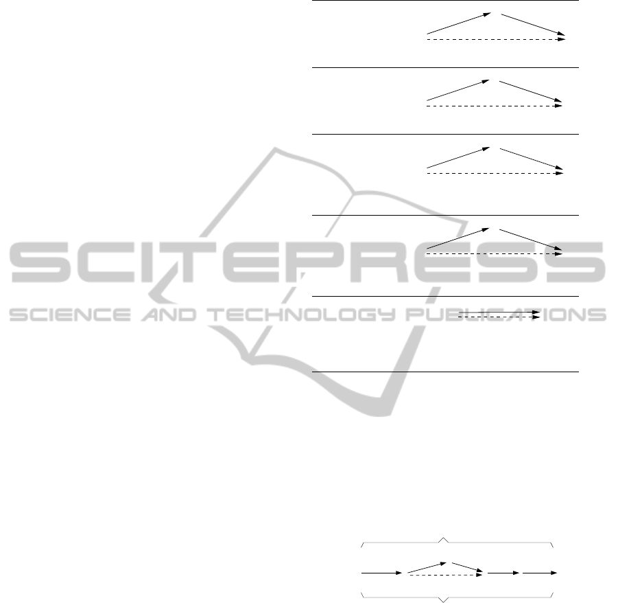
1.3.1 Edge-generation Rules
Intuitively, the ordinary constraints in an STNU are
constraints that the agent in charge of executing time-
points wants to satisfy. In contrast, the lower-case
and upper-case edges represent uncontrollable pos-
sibilities that could potentially threaten the satisfac-
tion of the ordinary constraints. Typically, to elim-
inate such threats, the agent must satisfy additional
constraints—or, in graphical terms, add new edges
to the graph. Toward that end, Morris and Muscet-
tola (2005) presented the five edge-generation rules in
Table 1, where pre-existing edges are denoted by solid
arrows and newly generated edges are denoted by
dashed arrows. The first four rules each take two pre-
existing edges as input and generates a single edge as
output. The Label-Removal rule takes only one edge
as input. Incidentally, applicability conditions of the
form, Y 6≡ Z, should be construed as stipulating that
Y and Z must be distinct time-point variables, not as
constraints on the values of those variables.
Note that the rules only generate new ordinary or
upper-case edges, never new lower-case edges. The
generated ordinary edges represent additional con-
straints that must be satisfied to avoid threatening the
satisfaction of the original constraints. The generated
upper-case edges represent additional conditional
constraints that the agent must satisfy. In particular,
a generated UC edge of the form, Y
−→
C :−w
A,
represents a conditional constraint that can be glossed
as: “As long as the contingent duration C − A might
take on its maximum value, then A −Y ≤ −w (i.e.,
Table 1: Edge-generation rules.
No Case:
S
T
Q
v
u
u +v
Upper Case:
S
T
Q
u
R: v
R: u +v
Lower Case:
S
T
Q
s: u
v
u +v
Applicable if: v < 0 or (v = 0 and S 6≡ T )
Cross Case:
S
T
Q
R: v
R: u +v
s: u
Applicable if: R 6≡ S and (v < 0 or (v = 0 and S 6≡ T ))
Label Removal:
S
T
v
R: v
Applicable if: v ≥ −x, where x is the lower
bound for the contingent link from T to R
Y ≥ A + w) must be satisfied”.
1.3.2 Path Transformations
Morris (2006) showed that the process of edge gen-
eration can also be viewed as one of path transfor-
mation or path reduction. For example, as illustrated
in Fig. 2, suppose a path P contains two adjacent
e
e
2
e
1
P
P
0
Figure 2: Transforming a path P into the path P
0
.
edges, e
1
and e
2
, to which one of the first four edge-
generation rules can be applied to generate a new edge
e. Let P
0
be the path obtained from P by replacing e
1
and e
2
by the new edge e. We say that P has been
transformed into (or reduced to) P
0
. Similarly, if P
contains a UC edge E to which the Label-Removal
rule can be applied to generate a new ordinary edge
E
o
, then P can be transformed by replacing E by E
o
.
Finally, any sequence of zero or more such transfor-
mations also counts as a path transformation. Fig. 3
illustrates the transformation of a path P using the
MagicLoopsinSimpleTemporalNetworkswithUncertainty-ExploitingStructuretoSpeedUpDynamicControllability
Checking
159

Q
R S
T
r : 5
3
U
P
0
P
3−2
−7
−10
Figure 3: A two-step transformation of a path P into P
0
.
No-Case rule followed by the Lower-Case rule.
An important property of path transformations is
that they preserve unlabeled length (i.e., the length of
the path ignoring any alphabetic labels on its edges).
This follows directly from the fact that each edge-
generation rule preserves unlabeled length.
Morris (2006) introduced semi-reducible paths,
which play a central role in the determination of dy-
namic controllability. For convenience, we present
the definition in terms of OU-edges and OU-paths.
Definition 1 (OU-edge, OU-path). An OU-edge is an
edge that is either ordinary or upper-case. An OU-
path is a path consisting solely of OU-edges.
Definition 2 (Semi-reducible path; SRN loop). A
path in an STNU graph is called semi-reducible if
it can be transformed into an OU-path. A semi-
reducible loop with negative unlabeled length is
called an SRN loop.
Note that the path, P , in Fig. 3 is semi-reducible since
it can be transformed into the OU-path, P
0
.
1.3.3 The N
4
DC-Checking Algorithm
The N
4
algorithm takes a two-step approach to de-
termining whether an STNU has any SRN loops. In
Step 1, it generates the OU-edges that could arise
from the transformation of semi-reducible paths into
OU-paths. The dashed edges in Fig. 3 are examples
of such edges. In Step 2, it gathers the OU-edges
from Step 1—minus any alphabetic labels—into an
STN, S
†
. It then computes the corresponding distance
matrix, D
†
, which turns out to equal the SR-distance
matrix, D
∗
, for the original STNU (i.e., the all-pairs,
shortest-semi-reducible-paths matrix).
To illustrate Step 1, consider a semi-reducible
path, P , that consists of original STNU edges, in-
cluding at least one lower-case edge e, as shown in
Fig. 4. Since P is semi-reducible, there must be some
sequence of reductions by which P is transformed
into an OU-path. Thus, sometime during that trans-
formation, the Lower-Case or Cross-Case rule must
be applied to e and some other edge e
0
to yield a new
OU-edge ˜e, effectively removing e from the path. We
say that e has been “reduced away”. To enable this,
e
e
0
P
e
˜e
Figure 4: Reducing away a lower-case edge, e.
the original path P must have a sub-path, P
e
, imme-
diately following e, such that P
e
reduces to the edge
e
0
, as shown in Fig. 4.
3
The concatenation of the LC
edge e with the sub-path P
e
is called a lower-case re-
ducing sub-path (LCR sub-path); edges such as ˜e that
are generated by transforming an LCR sub-path into a
single edge, are called core edges (Hunsberger, 2010).
In view of the above, it follows that every occur-
rence of a lower-case edge, e, in any semi-reducible
path, P, must belong to an LCR sub-path in P . Stated
differently, the edges in any semi-reducible path, P,
that do not belong to an LCR sub-path must be OU-
edges from the original STNU. Thus, Step 1 of the
N
4
algorithm searches for LCR sub-paths and the core
edges that they generate. Crucially, this search does
not require exhaustively applying the edge-generation
rules from Table 1. Instead, as will be seen, the search
can be limited to so-called extension sub-paths, which
have an important nesting property. At the end of
Step 1, the algorithm has a set, E, of OU-edges.
For Step 2, note that there is a one-to-one corre-
spondence between shortest semi-reducible paths in
the original STNU and shortest paths consisting of
edges in E. In particular, if P is a shortest semi-
reducible path, then it can be transformed into a path,
P
0
, whose edges are in E; and since path transfor-
mations preserve unlabeled length, |P | = |P
0
|. Simi-
larly, if P
0
is a shortest path with edges in E, then, by
“unwinding” the transformations that generated the
edges in E, P
0
can be “un-transformed” into a semi-
reducible path P , again, such that |P
0
| = |P|.
Next, since alphabetic labels are irrelevant to the
computation of unlabeled lengths, let E
†
be the set of
ordinary edges obtained by stripping any alphabetic
labels from the edges in E; let S
†
be the correspond-
ing STN; and let D
†
be the corresponding distance
matrix. Then D
†
is equal to the all-pairs, shortest-
paths matrix for paths with edges in E, and hence
D
†
= D
∗
. Thus, the N
4
algorithm concludes that the
original STNU is DC iff D
†
is consistent.
3
In Fig. 3, the LC edge from Q to R is reduced away by
the path from R to S to T , yielding an edge from Q to T.
ICAART2013-InternationalConferenceonAgentsandArtificialIntelligence
160

2 MODIFYING MORRIS’
ANALYSIS
To simplify his mathematical analysis, Morris (2006)
introduces two kinds of instantaneous reactivity into
the semantics of dynamic controllability. First, he
allows contingent links of the form, (A,0, y,C), in
which the lower bound on the contingent duration is
zero. This effectively allows scenarios in which it
is uncertain whether the temporal interval between a
cause and its effect will be instantaneous. Second, he
allows an agent to react instantaneously to an obser-
vation of a contingent execution. Although these sorts
of instantaneous reactions may be applicable to some
domains, this author prefers to stick with the more re-
alistic assumptions of the original semantics—and the
edge-generation rules in Table 1—in which both the
lower bounds of contingent durations and agent reac-
tion times must be positive. The rest of this section
shows how Morris’ concepts and techniques must be
modified to conform to the original semantics of dy-
namic controllability.
• For convenience, proofs for the results in the rest
of the paper are sketched in the Appendix.
Given his assumptions, Morris changed the condi-
tions for the Lower-Case rule to v < 0 (i.e., he elim-
inated the case, v = 0). The reason is that when
v = 0, the edge, S
−→
v
T , represents the con-
straint, T −S ≤ 0 (i.e., T ≤ S), which expresses that T
must execute no later than the contingent time-point
S. If able to react instantaneously, an agent need only
wait for S to execute and then instantaneously execute
T . Thus, no additional constraint is required to guard
against S executing early. If unable to react instan-
taneously, then the new edge from Q to T is needed.
Similar remarks apply to the Cross-Case rule.
Extension Sub-paths. Let e be some LC edge in a
path, P ; and let e
1
,e
2
,. .. be the sequence of edges
immediately following e in P. If e can be reduced
away in P , then it may be that there are many values
of m ≥ 1 for which the sub-path, e
1
,e
2
,. ..,e
m
, could
be used to reduce away e. For example, the LC edge
from Q to R in Fig. 3 can be reduced away not only
by the two-edge sub-path from R to T , as shown in
the figure, but also by the three-edge sub-path from R
to U . In such cases, the extension sub-path, defined
below, will turn out to be the sub-path that can reduce
away e for which the value of m is the smallest.
Definition 3 (Extension sub-path; moat edge). Let e
be an LC edge in a path P . Let e
1
,e
2
,. .. be the se-
quence of edges that immediately follow e in P . For
each i ≥ 1, let P
i
e
be the sub-path of P consisting of
the edges, e
1
,. ..,e
i
. If it exists, let m be the smallest
integer such that either:
(1) |P
m
e
| < 0; or
(2) |P
m
e
| = 0 and P
m
e
is not a loop.
4
Then the extension sub-path (ESP) for e in P, notated
P
e
, is the sub-path P
m
e
; and its last edge, e
m
, is called
the moat edge for e in P . If no such m exists, then e
has no ESP or moat edge in P .
For the LC edge from Q to R in Fig. 3, the extension
sub-path is the two-edge path labeled P
e
; and the moat
edge is the edge from S to T .
Structure of ESPs. Given the setup in Defn. 3, m is
the smallest value for which |P
m
e
| < 0 or P
m
e
is a zero-
length non-loop. Conversely, for any i < m, either
|P
i
e
| > 0 or P
i
e
is a zero-length loop. In turn, this im-
plies that any ESP must consist of zero or more loops
of length zero, followed by a (non-empty) sub-path
that does not have any prefixes that are zero-length
loops. These observations motivate the following.
Definition 4 (Pesky prefix; nice path). A pesky prefix
of P is a non-empty prefix of P that is a loop of length
0. A nice path is one having no pesky prefixes.
In general, an ESP may have zero or more pesky
prefixes, followed by a non-empty nice path.
5
Fig. 5
extension sub-path
A
C
X
1
C
X
2
X
3
C
2
4
X
4
X
5
1
−3
−6
−3
pesky prefix
nice suffix
c: 3
pesky prefix
lower-case
edge
3
Figure 5: An ESP with two pesky prefixes.
shows an ESP with two pesky prefixes, one nested
inside the other, followed by a non-empty nice suffix.
Nesting Property for ESPs. The following lemma
confirms that ESPs as defined in Defn. 3 have the nest-
ing property highlighted by Morris (2006).
Lemma 1 (Nesting Property for ESPs). Let P
1
and
P
2
be two ESPs within the same path P. Then P
1
and
P
2
are either disjoint (i.e., share no edges) or one is
nested inside (i.e., is a sub-path of) the other.
4
For Morris (2006), case (2) is not needed because he
eliminated the case, v = 0, from the applicability conditions
for the Lower-Case and Cross-Case rules.
5
Unlike Morris (2006), for whom every ESP has nega-
tive length, this paper must carefully distinguish pesky pre-
fixes from ESPs of length zero.
MagicLoopsinSimpleTemporalNetworkswithUncertainty-ExploitingStructuretoSpeedUpDynamicControllability
Checking
161

Breaches and Usable/Unusable Moat Edges. Sup-
pose that P is a path that contains an occurrence of
a lower-case edge, e, that derives from a contingent
link, (A, x,y,C). Thus, e has the form, A
−→
c: x
C.
Suppose further that e has an extension sub-path, P
e
,
in P . The existence of an ESP for e in P turns out to
be a necessary, but insufficient condition for reducing
away e in P . For example, using Fig. 4 as a refer-
ence, if the edge, e
0
, into which P
e
is transformed,
happens to be an upper-case edge with alphabetic la-
bel C (i.e., that matches the lower-case label on e),
then the Cross-Case rule cannot be applied to e and e
0
,
blocking the reducing away of e.
6
Such moat edges
are called unusable.
7
The following definitions spec-
ify the characteristics of usable/unusable moat edges.
Definition 5 (Breach; usable/unusable moat edge).
Let e be a lower-case edge corresponding to a contin-
gent link, (A,x,y,C); let P
e
be the ESP for e in some
path P ; and let e
m
be the corresponding moat edge.
Any occurrence in P
e
of an upper-case edge labeled
by C is called a breach. If P
e
has no breaches, then it
is called breach-free. If e
m
is a breach and |P
e
| < −x,
then e
m
is said to be unusable; otherwise, it is usable.
8
Theorem 3, below, shows the crucial role of usable
moat edges for semi-reducible paths (Morris 2006).
Theorem 3. A path P is semi-reducible if and only if
each of its lower-case edges has a usable moat edge.
Since a pesky prefix, by definition, has length
zero, extracting a pesky prefix from an extension sub-
path cannot affect its length. In addition, since a pesky
prefix cannot constitute the entirety of an extension
sub-path, extracting a pesky prefix cannot affect the
moat edge. Therefore, the usability of a moat edge
cannot be affected by extracting a pesky prefix from
an ESP and, hence, the semi-reducibility of a path
cannot be affected by extracting pesky prefixes.
Corollary 1. Let P be any path. Let P
0
be the path
obtained from P by extracting all pesky prefixes from
any extension sub-paths within P . Then P is semi-
reducible if and only if P
0
is semi-reducible.
Given this result, the rest of this paper presumes
that all pesky prefixes are extracted from any path
without affecting its semi-reducibility.
Corollary 2. Any semi-reducible path, P , can be
transformed into an OU-path using a sequence of re-
ductions whereby each LC edge e in P is reduced
away by its corrresponding extension sub-path P
e
.
6
Recall the condition, R 6≡ S, for the Cross-Case rule.
7
It could also be said that P
e
is unusable.
8
Morris (2006) converts STNUs into a normal form in
which the value of x is invariably zero.
Figure 6: A semi-reducible path with nested ESPs.
Fig. 6 illustrates a semi-reducible path with nested
extension sub-paths. In the figure, lower-case edges
are shown with a distinctive arrow type, ESPs are
shaded, and the core edges are dashed.
Morris (2006) proved that an STNU with K con-
tingent links has an SRN loop if and only if it has a
breach-free SRN loop in which extension sub-paths
are nested to a depth of at most K. Thus, his N
4
DC-checking algorithm performs K rounds of search-
ing for breach-free extension sub-paths that could be
used to reduce away lower-case edges, each round
effectively increasing the nesting depth of extension
sub-paths. The core edges generated in this way are
then collected—minus any upper-case labels—into an
STN, S
†
, as previously described, to compute the dis-
tance matrix, D
†
, which equals the all-pairs, shortest-
semi-reducible-paths matrix for the original STNU.
3 INDIVISIBLE SRN LOOPS
This section introduces a new approach to analyzing
the structure of semi-reducible negative loops. The
key feature of the approach is its focus on the number
of occurrences of lower-case edges in what it calls in-
divisible SRN loops (or iSRN loops). As will be seen,
for the purposes of DC checking, it suffices to restrict
attention to iSRN loops. However, the main result of
this section is that the number of occurrences of LC
edges in any iSRN loop in any STNU having K con-
tingent links is at most 2
K
− 1. Section 4 shows how
to construct STNUs that have iSRN loops—called
magic loops—that attain this upper bound. Section 5
exploits the 2
K
− 1 bound to speed up the DC check-
ing for some STNUs.
The measure of complexity considered below is
the number of occurrences of LC edges in a path.
Definition 6. For any path, P , the number of occur-
rences of lower-case edges in P is denoted by #P .
Suppose that P is an SRN loop and Q is a sub-
loop of P that also happens to be an SRN loop (i.e., Q
is an SRN sub-loop of P ). Since every LC edge in Q
also belongs to P , it follows that #Q ≤ #P . However,
if P is an indivisible SRN loop, then #Q must equal
#P . That is, no SRN sub-loop of an iSRN loop P can
have fewer occurrences of LC edges than P.
ICAART2013-InternationalConferenceonAgentsandArtificialIntelligence
162

This sub-loop is not semi-reducible.
This sub-loop has non-negative length.
B
E
C
D
−20
B
D
A
B
A
B
B: −20
b: 1
B: −20
10
D: −30
b: 1
30
d : 1
40
Figure 7: An indivisible SRN loop, P .
Definition 7 (iSRN loop). Let P be an SRN loop. P
is called an indivisible SRN loop (or iSRN loop) if
#Q = #P for every SRN sub-loop Q of P .
Fig. 7 shows an example of an SRN loop, P , that
has no SRN sub-loops and, thus, is indivisible. P con-
tains three occurrences of LC edges (shown with a
distinctive arrow style); that is, #P = 3. P is semi-
reducible because each LC edge has a correspond-
ing breach-free extension sub-path that can be used
to reduce it away. In addition, |P| = −7 < 0. Fi-
nally, although P has many sub-loops, two of which
are shaded in the figure, none of them are SRN sub-
loops. For example, the lefthand shaded sub-loop is
not semi-reducible and the righthand shaded sub-loop
is non-negative. Thus, P is an iSRN loop.
Lemma 2, below, shows that for DC checking, it
suffices to restrict attention to iSRN loops. The iSRN
loop, P
0
, is obtained by recursively extracting SRN
sub-loops until, eventually, an iSRN loop is found.
Lemma 2. If an STNU S has an SRN loop P , then
S also has an iSRN loop P
0
. Furthermore, P
0
can be
chosen such that #P
0
≤ #P .
The search for an upper bound on the number of
occurrences of LC edges in any iSRN loop begins by
focusing on root-level LCR sub-paths (i.e., LCR sub-
paths that are not contained within any other). This
notion can be defined since, by Lemma 1, ESPs in
any semi-reducible path must be disjoint or nested.
Definition 8 (Root-level). Let e be an occurrence of
an LC edge in a semi-reducible path P ; and let P
e
be
the extension sub-path for e in P . If P
e
is not con-
tained within any other ESP in P , then P
e
is called a
root-level ESP in P ; e is called a root-level LC edge
in P ; and the LCR sub-path formed by concatenating
e and P
e
is called a root-level LCR sub-path.
Theorem 4 bounds the number of root-level LCR
sub-paths in any iSRN loop.
Theorem 4. An iSRN loop in an STNU with K con-
tingent links has at most K root-level LCR sub-paths.
Theorem 5, below, bounds the depth of nesting of
LCR sub-paths (or, equivalently, ESPs) in an iSRN
loop. It extends Morris’ result that if an STNU with
K contingent links has an SRN loop, then it has a
breach-free SRN loop whose extension sub-paths are
nested to a depth of at most K.
Theorem 5. Let P be an iSRN loop in an STNU hav-
ing K contingent links. Then P is breach-free and has
LCR sub-paths nested to a depth of at most K.
Although Theorem 5 bounds the nesting depth of
LCR sub-paths in an iSRN loop, it does not limit the
number of LC edges within any root-level LCR sub-
path. Theorem 6, below, shows that in any non-trivial
iSRN loop there must be an LC edge that occurs ex-
actly once, and that that occurrence must be at the root
level.
Theorem 6. If P is an iSRN loop that contains at
least one lower-case edge, then P must have a root-
level LC edge that occurs exactly once in P.
This result provides the key for the inductive proof
of Theorem 7, below, the main result of this section.
Theorem 7. If P is an iSRN loop in an STNU with K
contingent links, then #P ≤ 2
K
− 1.
Finally, Theorem 8 shows that the ordinary edges
associated with contingent links (cf. Fig. 1) can be
ignored for the purposes of DC checking.
Theorem 8. Any STNU having an SRN loop has an
iSRN loop that contains none of the ordinary edges
associated with contingent links.
Although this does not affect the worst-case com-
plexity of DC checking, it has the potential to limit
the branching factor of edge generation in practice.
4 MAGIC LOOPS
Section 3 showed that the number of LC edges in
any iSRN loop is at most 2
K
− 1. This section de-
fines a magic loop as any iSRN loop that has exactly
2
K
− 1 occurrences of LC edges. It then presents an
algorithm for constructing such loops, thereby prov-
ing that the 2
K
− 1 bound is tight. Interestingly, the
STNUs used to generate these magic loops have only
2K + 1 time-points (two time-points for each contin-
gent link, plus one extra time-point) and 4K edges.
Definition 9 (Magic Loop). A magic loop of order K
is any iSRN loop that (1) belongs to an STNU having
K contingent links; and (2) contains exactly 2
K
− 1
occurrences of LC edges
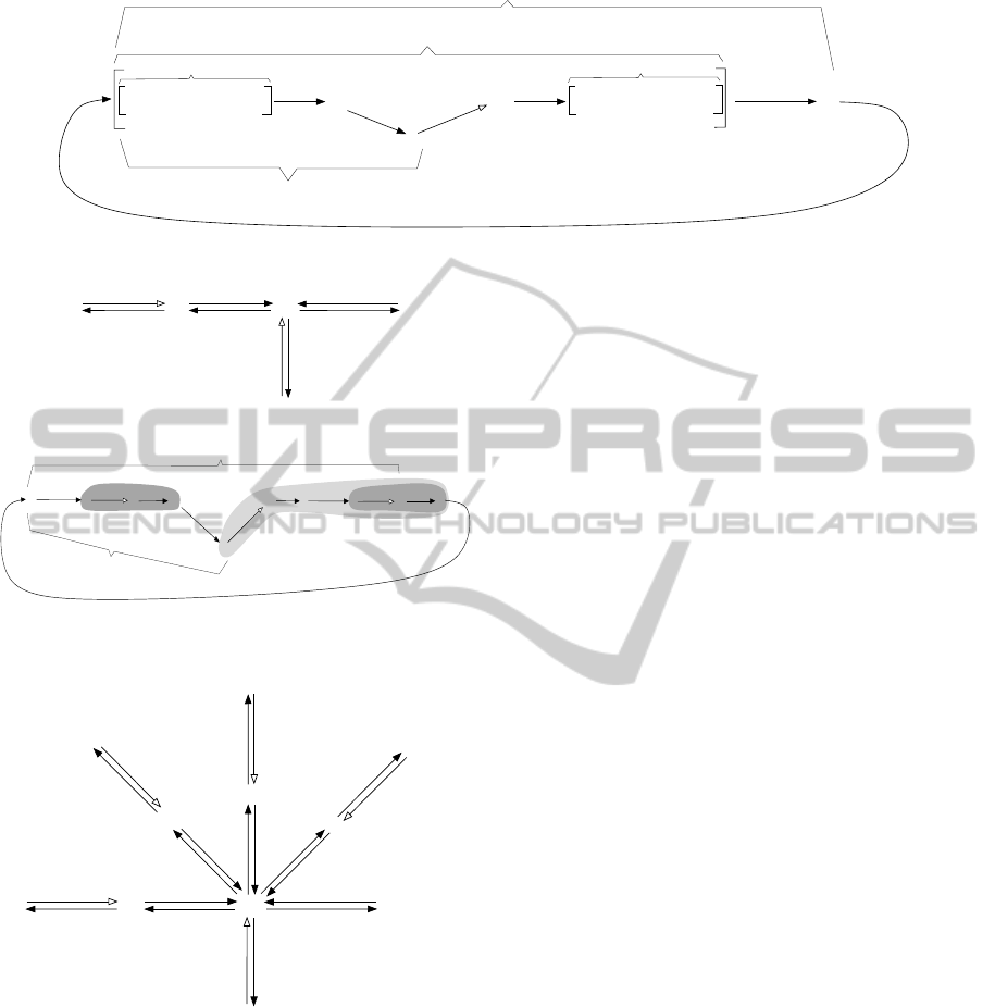
The algorithm for constructing magic loops is
recursive. For each K ≥ 1, it defines an STNU,
S
K
, that contains a magic loop, M
K
, of order K.
The STNUs and magic loops employ edges whose
lengths are specified by numerical parameters, such
MagicLoopsinSimpleTemporalNetworkswithUncertainty-ExploitingStructuretoSpeedUpDynamicControllability
Checking
163

as x
i
,y
i
,α
i
,β
i
,γ
i
, and δ
i
, where 1 ≤ i ≤ K. All of
these parameters have positive integer values; thus,
any negative values are specified with explicit nega-
tive signs, as in: −y
i
,−α
i
or −γ
i
. Each magic loop,
M
K
, also has several sub-paths, including φ
i
, χ
i
and
ω
i
. These sub-paths have important properties that
are exploited in the related proofs. It shall turn out
that all of the parameters are positive; however, the
lengths, |φ
i
|,|χ
i
| and |ω
i
| are invariably negative.
⇒ For convenience, the rest of this section uses k in-
stead of K, and ∗ instead of k + 1. Thus, for ex-
ample, S
∗
is shorthand for S
K+1
.
C
1
X
−1
A
1
C
1
:−3
c
1
:1
2
C
1
X
A
1
2
C
1
C
1
:−3
c
1
:1
−1
φ
1
ω
1
χ
1
Figure 8: The STNU S
1
(top) and magic loop M
1
(bottom).
X
δ
k
−γ
k
C
1
c
1
:x
1
C
1
:−y
1
A
1
and edges
time-points
additional
C
1
X
C
1
.......
.........
A
k
δ
k
−γ
k
χ
k
φ
k
ω
k
Figure 9: The generic form of S
k
(top) and M
k
(bottom).
For the base case, the STNU S
1
and its magic loop
M
1
are shown in Fig. 8. M
1
contains two sub-loops,
neither of which is an SRN loop; thus, it is an iSRN
loop. Also, M
1
contains 2
1
− 1 = 1 occurrence of an
LC edge; thus, it is a magic loop of order 1. For the
recursive case, we assume that we have S
k
, an STNU
with k contingent links that has the form shown
at the top of Fig. 9, and M
k
, a magic loop of order
k having the form shown at the bottom of Fig. 9. Note
that S
1
and M
1
have the desired forms.
In general, the values of γ
k
, |φ
k
| and |χ
k
| suffice to
generate the values of the parameters, α
∗
,β
∗
,γ
∗
,δ
∗
,x
∗
and y
∗
, which are determined sequentially, as shown
in Rules 1–6 of Table 2.
9
Once these values are in
hand, the STNU, S
∗
, is built out of S
k
as shown in
Fig. 10; and the magic loop, M
∗
, is created with the
9
Recall that the asterisk is used as a shorthand for k +1.
Table 2: Rules for generating parameters for the case k + 1.
(1) α
∗
= γ
k
(2) β
∗
= 1 − 2|φ
k
| + γ
k
(3) γ
∗
= 2 − 2|φ
k
| + |χ
k
| + γ
k
(4) δ
∗
= 2 − 3|φ
k
| + γ
k
(5) x
∗
= 1
(6) y
∗
= 3 − 3|φ
k
| + |χ
k
|
X
C
1
δ
∗
−γ
∗
A
1
C
1
:−y
1
c
1
:x
1
C
∗
−α
∗
β
∗
additional
time-points
and edges
for S
k
A
∗
c
∗
:x
∗
C
∗
:−y
∗
edges for S
∗
additional time-points and
Figure 10: Building the STNU, S
∗
, from S
k
.
structure shown in Fig. 11.
Notice, too, that M
∗
introduces a single, new
lower-case edge associated with a contingent link,
(A
∗
,x
∗
,y
∗
,C
∗
). Since each χ
k
sub-path has 2
k
− 1
occurrences of LC edges, the total number of occur-
rences of LC edges in M
∗
is 1+ 2(2
k
−1) = 2
k+1
−1,
as desired. Fig. 12 shows the STNU S
2
and magic
loop M
2
generated using these parameters; the LCR
sub-paths are shaded for convenience.
Although the structure of magic loops of higher
orders is extremely convoluted, the structure of the
corresponding STNU graphs is much simpler. For ex-
ample, the STNU, S
5
, is shown in Fig. 13.
Finally, Theorem 9, below, shows that for each
k ≥ 1, the loop, M
k
, is indeed a magic loop; and The-
orem 10 shows that for each k ≥ 1, the only iSRN
loops in S
k
are necessarily magic loops; thus, there
are no iSRN loops in S
k
having fewer than 2
k
− 1 oc-
currences of lower-case edges. Taken together, these
theorems show that magic loops are not only worst-
case scenarios in terms of the number of occurrences
of LC edges in an iSRN, but also that there are STNUs
for which this worst-case scenario is the only case.
Theorem 9. For each k ≥ 1, the loop, M
k
, is a magic
loop of order k (i.e., an iSRN loop having exactly
2
k
− 1 occurrences of lower-case edges).
Theorem 10. Let S
k
be the STNU as described in this
section for some k ≥ 1. Every SRN loop in S
k
has at
least 2
k
− 1 occurrences of LC edges.
5 SPEEDING UP DC CHECKING
This section presents a recursive O(N
3
)-time pre-
ICAART2013-InternationalConferenceonAgentsandArtificialIntelligence
164
...........
.........
χ
k
...........
.........
χ
∗
ω
∗
φ
∗
−γ
∗
X
δ
∗
χ
k
C
1
A
k
C
1
−α
∗
A
∗
β
∗
C
1
A
k
C
1
C
∗
:−y
∗
c
∗
:x
∗
C
∗
C
∗
Figure 11: The structure of M
∗
, a magic loop of order k + 1.
C
1
C
1
:−3
A
2
C
2
:−10
−1
8
A
1
−7
c
2
:1
C
2
c
1
:1
12
X
C
2
C
2
:−10
A
2
C
2
c
2
:1
χ
2
−1
C
1
A
1
C
1
c
1
:1
C
1
:−3
φ
2
8
C
1
C
1
:−3
A
1
c
1
:1
C
1
−7
X
12
Figure 12: STNU S
2
(top) and magic loop M
2
(bottom).
C
1
C
1
:−3
C
2
:−10
−1
8
A
1
c
2
:1
C
2
X
A
2
C
3
A
3
C
3
:−36
c
3
:1
C
4
A
4
A
5
C
5
:−470
c
1
:1
−399
648
c
4
:1
128
C
5
−109
c
5
:1
468
C
4
:−130
−29
34
−7
Figure 13: The STNU S
5
that contains the magic loop M
5
.
processing algorithm that exploits the 2
K
− 1 bound
on the number of occurrences of LC edges in iSRN
loops. For certain networks, this pre-processing algo-
rithm decreases the computation time for the N
4
DC-
checking algorithm from O(N
4
) to O(N
3
).
Let S be an STNU having K contingent links.
The pre-processing algorithm computes, for each con-
tingent time-point, C
j
, an upper bound on the num-
ber of distinct contingent time-points that can co-
occur in any iSRN loop in S that contains C
j
. The
largest of these upper bounds then serves as an upper
bound, UB, on the number of distinct contingent time-
points—and hence the number of distinct LC edges—
that can co-occur in any single iSRN loop in S. Since
any iSRN loop having at most UB distinct lower-case
edges can be viewed as an iSRN loop in an STNU
having exactly UB contingent links, such a loop can
have extension sub-paths nested to a depth of at most
UB (cf. Theorem 5). Thus, UB also provides an up-
per bound on the number of rounds needed for the N
4
algorithm to check the dynamic controllability of S.
In cases where UB < K, the pre-processing al-
gorithm can provide significant savings. Indeed, for
some STNUs, UB = 1, implying the need for only
one O(N
3
)-time round of the N
4
algorithm, even
though the unaware N
4
algorithm might still perform
K rounds at a cost of O(N
4
). At the other extreme,
for some STNUs, UB = K, in which case, the pre-
processing algorithm provides no benefit. However,
since the pre-processing algorithm runs in O(N
3
)
time, it does not introduce a significant overhead for
the N
4
algorithm, whose first step is an O(N
3
)-time
computation of a distance matrix.
In More Detail. Given an STNU, S , with K contin-
gent links, the algorithm begins by computing:
• 2
K
− 1, the maximum number of occurrences of
LC edges in any iSRN loop in S;
• ∆, the maximum value of y − x among all of the
contingent links, (A,x, y,C), in S; and
• D
, the all-pairs, shortest-path matrix for the OU-
paths in S , which can be computed in O(N
3
) time.
Next, for each pair of distinct contingent time-points,
C
i
and C
j
, it computes the value, LB
i j
:
LB
i j
= D
(C
i
,C
j
) + D
(C
j
,C
i
) − (2
K
− 1)∆.
As will be shown, if P is any iSRN loop in S that
contains both C
i
and C
j
, then |P | ≥ LB
i j
(i.e., LB
i j
is a Lower Bound for the lengths of iSRN loops that
contain both C
i
and C
j
). Thus, if LB
i j
≥ 0, it follows
that C
i
and C
j
cannot co-occur in any iSRN loop in S.
MagicLoopsinSimpleTemporalNetworkswithUncertainty-ExploitingStructuretoSpeedUpDynamicControllability
Checking
165

But in that case, any iSRN loop—if such exists—can
have at most K − 1 distinct LC edges and, thus, no
more than 2
(K−1)
− 1 occurrences of LC edges.
If the upper bound on the number of occurrences
of LC edges in iSRN loops in S can be lowered in this
way, the algorithm recursively seeks to identify ad-
ditional combinations of contingent time-points that
cannot co-occur within any iSRN loop. It terminates
when no further combinations can be found.
C
i
C
j
P
i j
P
ji
C
i
C
j
P
◦
i j
P
◦
ji
Figure 14: The iSRN loop, P, and its OU-cousin, P
◦
.
Consider the scenario in Fig. 14, where the left-
hand loop is an iSRN loop, P , that contains a pair
of distinct contingent time-points, C
i
and C
j
. Note
that the sub-path from C
i
to C
j
is called P
i j
, and the
sub-path from C
j
to C
i
is called P
ji
. Next, define the
ordinary cousin of an LC edge, A
−→
x
C, to be
the corresponding ordinary edge, A
−→
y
C, for the
contingent link (A,x,y,C) (cf. Fig. 1). The righthand
loop, P
◦
, in Fig. 14 is the same as P , except that any
occurrences of LC edges have been replaced by their
ordinary cousins. Since P
◦
may yet contain upper-
case edges, we call it the OU-cousin of P. Notice that
P
◦
is the concatenation of the OU-cousins of P
i j
and
P
ji
. Furthermore, since P
◦
i j
and P
◦
ji
are OU-paths, it
follows that their lengths are bounded below by the
corresponding OU-distance-matrix entries, whence:
D
(C
i
,C
j
) +D
(C
j
,C
i
) ≤ |P
◦
i j
| +|P
◦
ji
| = |P
◦
| (1)
Now, by Theorem 7, since P is an iSRN loop,
#P ≤ 2
K
− 1. Thus, the difference in the lengths of
P and P
◦
is bounded as follows:
∆
P
= |P
◦
|− |P| ≤ #P (2
K
−1)∆ ≤ (2
K
−1)∆ (2)
where ∆ is the maximum value of y − x over all the
contingent links in the STNU. Combining the in-
equalities (1) and (2) then yields:
|P | ≥ |P
◦
| − (2
K
− 1)∆
≥ D
(C
i
,C
j
) + D
(C
j
,C
i
) − (2
K
− 1)∆
Since this inequality must hold whenever P is
an iSRN loop in which the distinct contingent time-
points, C
i
and C
j
, both occur, it follows that if
D
(C
i
,C
j
) + D
(C
j
,C
i
) − (2
K
− 1)∆ ≥ 0
then there cannot be any such loop. (Recall that |P |
must be negative if P is an iSRN loop.)
Table 3: Pseudo-code for the pre-processing algorithm.
Given: An STNU S with K contingent links.
0. Initialization:
• Let ∆ and F be as defined in the text.
• For each i ∈ {1,2,. .. ,K},
◦ ctr
i
:= K; and
◦ Listy
i
:= a list of K entries, (i, j,F (i, j)), sorted
into decreasing order of the F (i, j) values.
• Q := the empty list.
1. Pop all entries off all Listy
i
lists for which
F (i, j) ≥ (2
ctr
i
− 1)∆.
2. While Q not empty:
a. Pop an entry, (i, j,F (i, j)), off of Q .
b. If (i, j) entry in F not yet crossed out:
i. Cross out the (i, j) entry in F .
ii. Decrement the counter, ctr
i
.
iii. Pop all entries, (i, j
0
,F (i, j
0
)), from Listy
i
for
which F (i, j
0
) ≥ (2
ctr
i
− 1)∆; push them onto Q .
c. Do Step b, above, for the entry, ( j, i,F ( j,i)).
3. Let UB = max{ctr
i
}.
Next, if for each pair of contingent time-points, C
i
and C
j
, we define F (i, j) = D
(C
i
,C
j
) + D
(C
j
,C
i
),
then the preceding rule, which is the main rule used
by the pre-processing algorithm, can be re-stated as:
• If C
i
and C
j
are distinct contingent time-points
such that F (i, j) ≥ (2
K
−1)∆, then C
i
and C
j
can-
not both occur in the same iSRN loop.
Pseudo-code for the pre-processing algorithm is
given in Table 3. For each contingent time-point, C
i
,
it defines the following variables:
• ctr
i
is an upper bound (initially ctr
i
= K) on the
number of distinct contingent time-points that can
co-occur in any iSRN loop that contains C
i
.
• Listy
i
is a list of entries from the i
th
row of the F
matrix, sorted into decreasing order.
As the algorithm runs, any entry, (i, j,F (i, j)) from
Listy
i
, for which F (i, j) ≥ (2
ctr
i
− 1)∆, signals that
C
j
could not occur in the same iSRN loop with C
i
.
Such entries are popped off Listy
i
and pushed onto
the global queue. As each entry from the global
queue is processed, the corresponding ctr
i
value de-
creases, which may lead to further entries moving
from Listy
i
to the global queue. The algorithm termi-
nates whenever the global queue is emptied, at which
point no further reductions in ctr
i
values can be made.
The algorithm returns the maximum ctr
i
value, which
specifies the maximum number of distinct contingent
time-points that can co-occur in any iSRN loop in
the given STNU. The Appendix proves that the algo-
rithm’s worst-case running time is O(N
3
).
ICAART2013-InternationalConferenceonAgentsandArtificialIntelligence
166

In best-case scenarios, the pre-processing algo-
rithm will result in all off-diagonal entries in F be-
ing crossed out, implying that there can be no nesting
of LCR paths in any iSRN loop. In such cases, it is
only necessary to do a single, O(N
3
)-time round of
the N
4
algorithm to ascertain whether the STNU is
dynamically controllable. The benefit in such cases
can be dramatic, for if the network contains even one
semi-reducible path having K levels of nesting, then
the unaided N
4
algorithm would needlessly perform
K rounds of processing in O(N
4
) time.
6 CONCLUSIONS
This paper presented a new way of analyzing the
structure of STNU graphs with the aim of speeding
up DC checking. It proved that the number of oc-
currences of lower-case edges in any iSRN loop is
bounded above by 2
K
− 1. It presented a recursive
algorithm for constructing STNUs that contain iSRN
loops that attain this upper bound, thereby showing
that the bound is tight. In view of their highly con-
voluted structure, such loops are called magic loops.
Finally, it presented an O(N
3
)-time pre-processing al-
gorithm that exploits the 2
K
−1 bound to speed up DC
checking for some networks. Thus, the paper makes
both theoretical and practical contributions.
Other researchers have sought to speed up the
process of DC checking using incremental algo-
rithms. Stedl and Williams (2005) developed Fast-
IDC, an incremental algorithm that maintains the dis-
patchability of an STNU after the insertion of new
constraints or the tightening of existing constraints.
Shah et al. (2007) extended Fast-IDC to accommo-
date the removal or weakening of constraints. Al-
though intended to be applied incrementally, their al-
gorithm showed orders of magnitude improvement
over an earlier pseudo-polynomial DC-checking algo-
rithm when evaluated empirically, checking dynamic
controllability from scratch. It would be interesting
to see if their work could be applied to generate an
incremental version of the Morris’ N
4
algorithm.
Others have extended the concept of dynamic con-
trollability to accommodate various combinations of
probability, preference and disjunction. For exam-
ple, Tsamardinos (2002) augmented contingent dura-
tions with probability density functions and provided
a method that, under certain restrictions, finds “the
schedule that maximizes the probability of execut-
ing the plan in a way that respects the temporal con-
straints.” Tsamardinos et al. (2003) then extended that
work by developing algorithms to compute lower and
upper bounds for the probability of a legal plan exe-
cution. Morris et al. (2005) similarly used probability
density functions to represent the uncertainties associ-
ated with contingent durations, but also incorporated
preferences over event durations. Rossi et al. (2006)
presented a thorough treatment of STNUs augmented
with preferences (but not probabilities). They defined
the Simple Temporal Problem with Preferences and
Uncertainty (STPPU) and notions of weak, strong and
dynamic controllability.
Effinger et al. (2009) defined dynamic controlla-
bility for temporally-flexible reactive programs that
include the following constructs: “conditional execu-
tion, iteration, exception handling, non-deterministic
choice, parallel and sequential composition, and sim-
ple temporal constraints”. They presented a DC-
checking algorithm for temporally-flexible reactive
programs that frames the problem as an “AND/OR
search tree over candidate program executions.”
REFERENCES
Cormen, T. H., Leiserson, C. E., Rivest, R. L., and Stein, C.
(2009). Introduction to Algorithms. MIT Press.
Dechter, R., Meiri, I., and Pearl, J. (1991). Temporal con-
straint networks. Artificial Intelligence, 49:61–95.
Effinger, R., Williams, B., Kelly, G., and Sheehy, M. (2009).
Dynamic controllability of temporally-flexible reac-
tive programs. In Gerevini, A., Howe, A., Cesta, A.,
and Refanidis, I., editors, Proceedings of the Nine-
teenth International Conference on Automated Plan-
ning and Scheduling (ICAPS 09). AAAI Press.
Hunsberger, L. (2010). A fast incremental algorithm for
managing the execution of dynamically controllable
temporal networks. In Proceedings of the 17th Inter-
national Symposium on Temporal Representation and
Reasoning (TIME-2010), pages 121–128, Los Alami-
tos, CA, USA. IEEE Computer Society.
Morris, P. (2006). A structural characterization of temporal
dynamic controllability. In Principles and Practice of
Constraint Programming (CP 2006), volume 4204 of
Lecture Notes in Computer Science, pages 375–389.
Springer.
Morris, P., Muscettola, N., and Vidal, T. (2001). Dynamic
control of plans with temporal uncertainty. In Nebel,
B., editor, 17th International Joint Conference on Ar-
tificial Intelligence (IJCAI-01), pages 494–499. Mor-
gan Kaufmann.
Morris, R., Morris, P., Khatib, L., and Yorke-Smith, N.
(2005). Temporal constraint reasoning with prefer-
ences and probabilities. In Brafman, R. and Junker,
U., editors, Proceedings of the IJCAI-05 Multidisci-
plinary Workshop on Advances in Preference Han-
dling, pages 150–155.
Rossi, F., Venable, K. B., and Yorke-Smith, N. (2006). Un-
certainty in soft temporal constraint problems: A gen-
eral framework and controllability algorithms for the
fuzzy case. Journal of Artificial Intelligence Research,
27:617–674.
MagicLoopsinSimpleTemporalNetworkswithUncertainty-ExploitingStructuretoSpeedUpDynamicControllability
Checking
167

Shah, J., Stedl, J., Robertson, P., and Williams, B. C.
(2007). A fast incremental algorithm for maintaining
dispatchability of partially controllable plans. In Mark
Boddy et al., editor, Proceedings of the Seventeenth
International Conference on Automated Planning and
Scheduling (ICAPS 2007). AAAI Press.
Stedl, J. and Williams, B. C. (2005). A fast incremental
dynamic controllability algorithm. In Proceedings of
the ICAPS Workshop on Plan Execution: A Reality
Check, pages 69–75.
Tsamardinos, I. (2002). A probabilistic approach to robust
execution of temporal plans with uncertainty. In Vla-
havas, I. P. and Spyropoulos, C. D., editors, Proceed-
ings of the Second Hellenic Conference on AI (SETN
2002), volume 2308 of Lecture Notes in Computer
Science, pages 97–108. Springer.
Tsamardinos, I., Pollack, M. E., and Ramakrishnan, S.
(2003). Assessing the probability of legal execution
of plans with temporal uncertainty. In Proceedings
of the ICAPS-03 Workshop on Planning under Uncer-
tainty and Incomplete Information.
Vidal, T. and Ghallab, M. (1996). Dealing with uncertain
durations in temporal constraint networks dedicated to
planning. In Wahlster, W., editor, 12th European Con-
ference on Artificial Intelligence (ECAI-96)”, pages
48–54. John Wiley and Sons, Chichester.
APPENDIX
Proof Sketches
Lemma 1 Proof. Each extension sub-path consists
of zero or more loops of length zero followed by a
nice suffix. By the definition of an ESP, each of
those building blocks satisfies the positive-proper-
prefix and negative-proper-suffix properties. Thus,
any LC edge belonging to one of those building-block
sub-paths must have an extension sub-path within
that same building block. Thus, if P
1
and P
2
are
ESPs within a single path P whose intersection is
non-empty, then one must be contained within the
other.
Theorem 3 Proof. Suppose P is a path such that
every LC edge in P has a usable moat edge. By
Lemma 1, extension sub-paths in P are either disjoint
or nested. Consider an LC edge e whose ESP P
e
is in-
nermost (i.e., does not contain any other ESP). Then
P
e
must be an OU-path. By definition of ESP, ev-
ery proper prefix of P
e
has non-negative length and,
thus, any upper-case edges they might reduce to can
have their labels removed by the Label-Removal rule.
Thus, P
e
itself can be reduced to a single OU-edge, e
0
.
Since P
e
’s moat edge is usable, |e
0
| > −x and, thus,
if e
0
is a breach, its upper-case label can be removed
by the Label-Removal rule. Continuing this process
recursively will reduce away all LC edges from P .
Thus, P is semi-reducible.
Going the other way, suppose that P is a path with
at least one LC edge, e, that does not have a usable
moat edge. If e does not have an ESP, then e can-
not be reduced away. Alternatively, if e has an ESP,
P
e
, whose moat edge, e
m
is unusable, then |P
e
| < −x
and e
m
is a breach. In that case, P
e
will reduce away
to a UC edge whose label cannot be removed by the
Label-Removal rule, thereby preventing e from being
reduced away.
Corollary 1 Proof. The usability of a moat edge can-
not be affected by extracting a pesky prefix from an
ESP.
Corollary 2 Proof. The recursive procedure used in
the first part of the proof of Theorem 3 shows how to
use the corresponding extension sub-paths to reduce
away any LC edges from a semi-reducible path, start-
ing with innermost ESPs and working outward.
Lemma 2 Proof. If P is an SRN loop that is not indi-
visbile, then it has an SRN sub-loop Q having fewer
occurrences of LC edges. Recursively extracting SRN
sub-loops in this way cannot continue for more than
#P steps and, thus, must eventually yield an iSRN
loop.
Theorem 4 Proof. Let P be an iSRN loop in an
STNU having K contingent links. Let e
1
,. ..,e
n
be the root-level LC edges in P ; and `
1
,. ..,`
n
the corresponding root-level LCR sub-paths. By
Lemma 1, these sub-paths are disjoint. By Corol-
lary 2, these LCR sub-paths can be reduced to core
edges, E
1
,. ..,E
n
. Let P
0
be the OU-path obtained
from P by replacing the root-level LCR sub-paths by
their corresponding core edges. If any e
i
and e
j
were
occurrences of the same LC edge, then P
0
could be
split into sub-loops, P
0
1
and P
0
2
, one containing E
i
,
the other containing E
j
. Since P is an iSRN loop
and |P | = |P
0
1
| + |P
0
2
|, |P
0
1
| < 0 or |P
0
2
| < 0. Without
loss of generality, suppose |P
0
1
| < 0. Replacing the
core edges in P
0
1
by the corresponding LCR sub-paths
yields an SRN sub-loop of P having fewer occur-
rences of LC edges, contradicting that P is an iSRN
loop.
Interlude. Morris (2006) used a technique of extract-
ing a sub-loop from a semi-reducible path while pre-
serving its semi-reducibility. The following lemma
specifies general conditions that suffice for such an
operation to succeed.
Extra Lemma A. Let P be a semi-reducible path that
contains a sub-loop, S, such that: (1) |S| ≥ 0; (2) every
ESP in P that contains S, but whose corresponding
ICAART2013-InternationalConferenceonAgentsandArtificialIntelligence
168

LC edge is not in S, is breach-free; and (3) S does not
contain any suffix of any ESP in P whose correspond-
ing LC edge is not in S. Then the path, P
0
, formed by
extracting S from P is semi-reducible with |P
0
| ≤ |P |.
Proof of Extra Lemma A. Since |S| ≥ 0, |P
0
| ≤
|P |. Thus, it only remains to show that P
0
is semi-
reducible. Let e be any LC edge in P
0
. Since e also
belongs to P , and P is semi-reducible, it follows that
e must have an ESP, P
e
, in P that can be used to re-
duce away e in P.
Now, since e is in P
0
, e cannot be in S. Thus,
by condition (3), S cannot contain any suffix of P
e
.
Thus, either P
e
does not intersect S or P
e
contains all
of S. In the first case, P
e
is a sub-path of P
0
and thus
can be used to reduce away e in P
0
too. Hence, e
has a usable moat edge in P
0
. In the second case, the
moat edge and possibly some of its predecessor edges
in P
e
cannot be contained in S. Now, extracting the
non-negative sub-loop S from P
e
may cause an earlier
edge in P
e
− S to become the new moat edge for e in
P
0
. However, by condition (2), P
e
cannot contain any
breaches; hence the moat edge for e in P
e
− S ⊆ P
0
must be usable. Since e was an arbitrary LC edge in
P
0
, P
0
must be semi-reducible by Theorem 3.
Theorem 5 Proof. First, if P contains a breach, let P
e
be an outermost breach-containing ESP for some LC
edge e corresponding to a contingent link, (A,x,y,C).
(Recall that ESPs must be nested or disjoint.) Let B
e
be the rightmost breach edge in P
e
. Then B
e
is a UC
edge labeled by C and terminating in the activation
time-point A. Let S be the sub-loop from the starting
time-point of the LC edge e to the ending time-point
of the UC edge B
e
. Since S is a prefix of P
e
, |S| ≥
0. Let P
0
be the path obtained from P by extracting
the sub-loop S. Conditions (2) and (3) of the Extra
Lemma can also be shown to hold for S. Thus, P
0
must be an SRN loop containing fewer occurrences
of LC edges that P , contradicting that P is an iSRN
loop.
Next, suppose the depth of nesting of ESPs in P
is more than K. Then P must have an occurrence of
some LC edge e whose corresponding ESP, P , con-
tains another occurrence of e. Let S be the prefix of
P
e
whose final edge is that second occurrence of e.
Then S is a non-negative sub-loop. Let P
0
be as in
the Extra Lemma. Conditions (2) and (3) of the Extra
Lemma can then be shown to hold. Thus, P
0
must be
an iSRN loop having fewer occurrences of LC edges
than P , contradicting that P is an iSRN loop.
Theorem 6 Proof. Suppose, contrary to the theorem,
that every LC edge in some iSRN loop P occurs more
than once. Let e
1
be some root-level LC edge. By the
proof of Theorem 5, e
1
cannot occur within its own
root-level LCR sub-path; and, by the proof of The-
orem 4, e
1
cannot occur more than once at the root-
level. Thus, a second occurrence of e
1
must occur in
the interior of some other root-level LCR sub-path for
some root-level LC edge e
2
. Similarly, a second oc-
currence of e
2
must occur in the interior of some other
root-level LCR sub-path for some root-level LC edge
e
3
. And so on. Since there are at most K distinct LC
edges in P , this pattern of inclusion must circle back
on itself.
Let ˆe
1
, ˆe
2
,. .., ˆe
v
be the root-level LC edges in this
cycle, listed in their order of appearance in P . (Since
P is a loop, this listing is not unique.) Thus, ˆe
2
is con-
tained in the root-level LCR sub-path for ˆe
1
, ˆe
3
is con-
tained in the root-level LCR sub-path for ˆe
2
, and so
on. Chop P into 2v pieces, ρ
1
,σ
1
,ρ
2
,σ
2
,. ..,ρ
v
,σ
v
,
where the first edge of each ρ
i
is the LC edge ˆe
i
; and
the first edge of each σ
i
is the occurrence of ˆe
i−1
in
the LCR sub-path for ˆe
i
. (We take ˆe
0
to represent ˆe
v
.)
By construction, |ρ
i
| > 0; thus,
∑
|ρ
i
| > 0.
Next, for each i, let ψ
i
be the sub-path whose first
edge is the interior occurrence of ˆe
i
and whose last
edge is the edge in P that precedes the root-level oc-
currence of e
i
. By construction, each ψ
i
is a semi-
reducible loop with #ψ
i
< #P ; thus, since P is an
iSRN loop, |ψ
i
| ≥ 0 for each i and
∑
|ψ
i
| ≥ 0. Fi-
nally, by permuting these sub-paths, it can be shown
that
∑
|ψ
j
| =
∑
|σ
j
| + m|P| for some integer m > 0.
But then |P | ≥ 0, contradicting that P is an iSRN
loop.
Theorem 7 Proof. By induction on K. For the base
case, K = 0 and thus there are 2
0
− 1 = 0 occurrences
of LC edges in every iSRN loop. For the recursive
case, suppose that every iSRN loop in an STNU with
K contingent links has at most 2
K
− 1 occurrences of
LC edges. Suppose that P is an iSRN loop in an
STNU with K + 1 contingent links. By Theorem 6,
P must contain some LC edge, e, that occurs at most
once in P, and that that occurrence must be at the root
level. Let ` be the root-level LCR sub-path for e in P;
and let E be the core edge that ` can be transformed
into.
Let P
1
be the path obtained from P by replacing
` by the core edge E. Since the only occurrence of e
in P was in `, e does not occur in P
1
. Next, let P
0
1
be
obtained from P
1
by removing any upper-case labels
from its upper-case edges that match the lower-case
label on e. By construction, P
0
1
does not contain e
or any matching UC edges; thus, it can be viewed as
a path in an STNU having only K contingent links.
Furthermore, |P
0
1
| = |P | < 0. It can be shown that
P
0
1
is an iSRN loop in an STNU having K contingent
links; and therefore that #P
0
1
≤ 2
K
− 1.
MagicLoopsinSimpleTemporalNetworkswithUncertainty-ExploitingStructuretoSpeedUpDynamicControllability
Checking
169

For the next part of the proof, let e be the root-
level LC edge described above; and let P
e
be its root-
level ESP. Then, let P
2
be the loop formed by P
e
and
a single new edge e
α
. By construction, if P
e
is a sub-
path from C to some time-point X, then e
α
is a new
edge from X back to C. The length of this new edge,
e
α
, is determined as follows:
• If P
e
does not have any negative-length sub-loops,
then |e
α
| = |P | − |P
e
| (i.e., the length of the por-
tion of P that e
α
is effectively replacing).
• Otherwise, let |e
α
| = M − |P
e
|, where M =
max{|S| : S is a negative sub-loop of P
e
}.
By construction, the only occurrence of e in P has
been extracted and, thus, does not appear in P
2
. In
addition, since P is an iSRN loop, P
e
cannot have
any breaches; thus, there are no occurrences of UC
edges in P
e
labeled by C. Thus, P
2
can be viewed
as a loop in an STNU having K contingent links. It
can be shown that P
2
is an iSRN loop; and thus that
#P
2
≤ 2
K
− 1. Finally,
#P =≤ (2
K
−1)+ 1 + (2
K
−1) = 2
(K+1)
−1.
Theorem 8 Proof. Let P be an iSRN loop. By The-
orem 5, P must be breach-free. Suppose that P con-
tains an occurrence of an ordinary edge, A
−→
y
C,
associated with a contingent link, (A,x,y,C). Call
this edge e
◦
. Let e be the corresponding LC edge,
A
−→
c: x
C. We shall show that P can be converted
into an SRN loop P
†
by replacing or removing the
offending occurrence of e
◦
.
First, let P
x
be the same as P except that the oc-
currence of e
◦
has been replaced by the LC edge e. If
P
x
is semi-reducible, then let P
†
= P
x
. Otherwise, the
non-semi-reducibility of P
x
must be due to the inclu-
sion of the LC edge e. That LC edge must have an
unusable moat edge (i.e., it must have a breach moat
edge, B
e
, with |P
e
| < −x). This implies that there
must be a sub-loop, S, from A to A in P . The first
edge of S is e
◦
; its last edge is B
e
. Let P
†
be obtained
by extracting the sub-loop S from P. Since S con-
tains the offending occurrence of e
◦
, it follows that
P
†
does not. The conditions of Extra Lemma A can
be shown to hold for S. Thus, P
†
is an SRN loop. If
P
†
happens not to be indivisible, then SRN sub-loops
can be extracted (as in the proof of Lemma 2) until
indivisibility is restored. Recursively removing any
remaining ordinary edges associated with contingent
links produces the result.
The case of the other kind of ordinary edge (cf.
Fig. 1) associated with contingent links is handled
similarly.
Note. Because Theorems 9 and 10 are not needed for
the rest of the paper, their proofs are omitted for space
reasons.
Proof that Pre-processing Algorithm Runs in
O(N
3
) Time. Step 0, which happens only once, is
dominated by the computation of the OU-distance
matrix, D
, which can be done in O(N
3
) time, for ex-
ample, using the Floyd-Warshall algorithm (Cormen
et al., 2009). Sorting K lists of K entries can be done
in O(K
2
logK) time, for example, using K runs of the
MergeSort algorithm (Cormen et al., 2009).
Step 1, which happens only once, involves scan-
ning no more than K
2
entries; thus, it can be done in
O(K
2
) time.
The while loop in Step 2 runs at most K(K − 1)/2
times. All subsidiary steps, except Step 2b(iv) can be
done in constant time. Thus, ignoring Step 2b(iv), all
of the iterations of the while loop in Step 2 can be
done in O(N
2
) time. As for Step 2b(iv), each entry
in the Listy
i
lists can only be popped/pushed once;
thus, the total number of pop/pushes from Step 2b(iv)
is order O(K
2
). In addition, each time through Step
2b(iv), the stopping condition is hit only once. Thus,
the total number of stoppings in Step 2b(iv) is O(K
2
).
Thus, Step 2, in its totality, is O(K
2
).
Since Step 3 is O(K), the overall worst-case time
complexity of the pre-processing algorithm is O(N
3
).
ICAART2013-InternationalConferenceonAgentsandArtificialIntelligence
170
