
Application of Edge and Line Detection to Detect the near Surface
Anomalies in Potential Data
Lenka Kosková Třísková and Josef Novák
The Institute of Novel Technologies and Applied Informatics, Technical University in Liberec, Studentská 2,
Liberec, Czech Republic
Keywords: Edge Detection, Field Anomaly Detection, Potential Field Data, Gravity.
Abstract: Presented paper is focused on fast near surface anomaly detection in potential data. Our aim is to find fast
and semi –automated anomaly detection technique for the near surface anomalies with defined geometry.
The proposed algorithm is based on the shape recognition. The edge and line detection is used on acquired
data to detect the typical shape of the anomaly. Shape geometry parameters are converted into the anomaly
parameters and location information. The technique was tested using a set of noise-free and noisy synthetic
gravity data; satisfactory results were obtained.
1 INTRODUCTION
The general idea of presented algorithm is to speed
up the initial search processes after an event such as
flooding or earthquake with the geophysical
methodology. We face a set of limitations: time,
hardware, power and network accessibility is
limited. The operation itself runs in unstable and
dangerous circumstances. Finally – after the disaster,
no fully qualified geophysical specialist is available
on site. Any semi-automated data pre-processing is
very useful in such situation.
In described application, there is no interest in
the detailed 3D model of the subsurface materials.
The main interest is in local anomalies with typical
characteristics, such as cavities in dams.
Desired algorithm should be able to answer
questions: What is a probability of presence of a
significant anomaly with defined density and
geometry in the current data? If it is present, where
is it located?
According to the application constraints, we are
interested to detect the anomalies near the surface –
the depth fits into the range from 0 to 50 m. The
highest detection accuracy is expected in the depth
interval from 0 to 20 m. Typical search pattern is an
object with contrast density (a cavity filled by air or
water), contrast resistivity (the buried infrastructural
networks).
The initial methodology testing was made using
analytical data for the spherical and cylindrical
gravity anomaly (in both vertical and horizontal
position).
The desired anomaly forms typical shapes in the
acquired data. Anomaly with sphere-like geometry
gives circle contours in data, wires, pipes and similar
geometries lead to lines in data.
Due to application constraints we are looking for
the fast and simple process. The presented
application is therefore based on smoothing (Shih,
2010), morphological processing (Shih, 2010), shape
detection and finally anomaly classification. The
algorithm works well for all tested geometries.
For future enhancement and more complex
anomaly geometry, we plan to use CNN support for
the shape classification (Aydogan, 2012; Li et al.,
2011) or textural analysis (Cooper, 2004).
All the presented algorithms were implemented
and tested in the Matlab software.
2 THEORY AND METHODS
2.1 The Anomaly
A general function presenting a symmetric potential
field anomaly can be expressed by simple equation
(Salem, 2011):
(1)
F is an amplitude factor, q is a shape factor
characterizing the shape of the anomaly. The r is the
693
Kosková T
ˇ
rísková L. and Novák J..
Application of Edge and Line Detection to Detect the near Surface Anomalies in Potential Data.
DOI: 10.5220/0004261206930696
In Proceedings of the 2nd International Conference on Pattern Recognition Applications and Methods (PRG-2013), pages 693-696
ISBN: 978-989-8565-41-9
Copyright
c
2013 SCITEPRESS (Science and Technology Publications, Lda.)
distance from the middle point of the anomaly to the
observation point on the surface. Detailed summary
of q and F values for different simple geometrical
bodies both for gravity and magnetic sources is
given for example in Salem (2011); in short it is
presented in Table 1. More complex anomaly
geometry can be derived from theory presented in
the Blakely (pages 192-213).
Table 1: The F and q factor for simple geometrical bodies,
gravity field (γ is gravitational constant, M is mass for the
sphere and density contrast times cross-sectional area for
the cylinder).
Anomaly type F q
Sphere γMz 3/2
Horizontal cylinder 2γMz 1
Vertical cylinder γM 0.5
Considering simple anomaly bodies, the f
function is a smooth function; maximum value is
located above the anomaly center. If the anomaly
field is presented as 2D image, it gives spherical
contours for sphere and vertical cylinder, for
horizontal cylinder we obtain linear contours.
For all three bodies a linear dependency between
the depth of anomaly center (z) and the surface
location of the half-maximum value (
.
:
.
.
(2)
The k value differs with anomaly type and its value
can be extracted directly from the equation (1)
(Mares, 1990; pages 55-57). The z value can be later
used to estimate the density (or mass) of the
anomaly directly from the equation (1).
Table 2: The value of the k parameter for different
anomaly types.
Anomaly type K
Sphere 1.305
Horizontal cylinder 1
Vertical cylinder
√
3
3
2.2 The Detection Process
The detection process itself contains following steps
(all the steps are described deeply later in the text):
1. The noise level enhancement based on
histogram analysis (optional).
2. Smoothing, if noise is detected (optional).
3. The detection of areas with value close to
maximum and half maximum.
4. Conversion of the maximum and half maximum
matrices into black and white pictures.
5. Line detection in maximum matrix – a line
significant for horizontal cylinder. The detection
of sphere and vertical cylinder is started
otherwise.
6. Shape detection in half maximum matrix to
measure the appropriate
.
value using the
maximum and half maximum matrix.
7. The parameters estimation and calculation of
estimated anomaly field. If no lines detected in
the image, both spherical and cylindrical fields
are calculated and compared with original
image – the closest shape is selected.
2.3 Noise and Smoothing
The noise in general can have a lot of sources (from
measurement errors to the noise of the measurement
equipment or the influence of the deeper anomalies).
In our application, the noise is simulated as a white
noise with selected level, which is added to the
original analytical data.
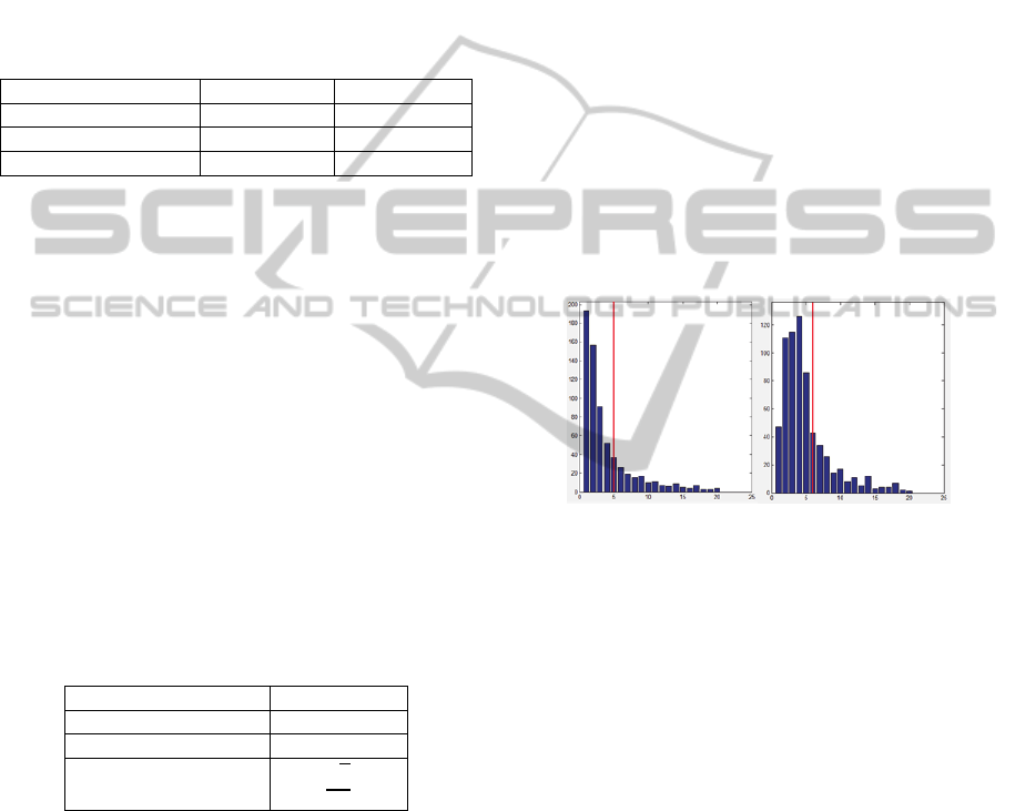
Figure 1: The histogram of a noise free spherical anomaly
(left picture) and noisy spherical anomaly (right picture,
noise level is from 0 to 0.2 of the maximum value).
All analytical data have very typical histogram,
which is depicted in Figure 1 on the left. The biggest
set of data has value close to the minimum. The
mean value is also closer to the minimum. The peak
at the minimum value is typical for higher mass and
small depth. (For the horizontal cylinder, most of the
values are less than a mean value of data.) White
noise has all values equally distributed between the
minimum and maximum value; the mean value is in
the middle of the maximum and minimum. By
general, each desired anomaly has its typical
histogram shape which can be tested on input data.
The histogram itself is not a key to determine the
anomaly shape. It can help to detect the noise and to
separate “nonsense” data without any searched
anomaly shape.
If a noise is detected the smooth filter is used.
The 3x3 and 5x5 averaging and Gauss smoothing
kernels were applied (Shih, 2010; page 52), best
results were obtained with averaging 3x3 filter. If
ICPRAM2013-InternationalConferenceonPatternRecognitionApplicationsandMethods
694
the histogram shows high noise level in the data, the
smoothing is repeated from 2 to 3 times.
2.4 Shape Detection
In the next step the maximum and half maximum
matrix is created: All the values higher than 98 % of
the maximum are colored in white, other left black
in the maximum matrix (MM). All the values higher
than 50 % of the maximum are white in the half
maximum matrix (HM).
Line detection process is now necessary to
distinguish the horizontal cylinder and other
anomalies – it is necessary to set up the thresholds of
following erosion process. We use the standard
Hough transform according to the Matlab (2009).
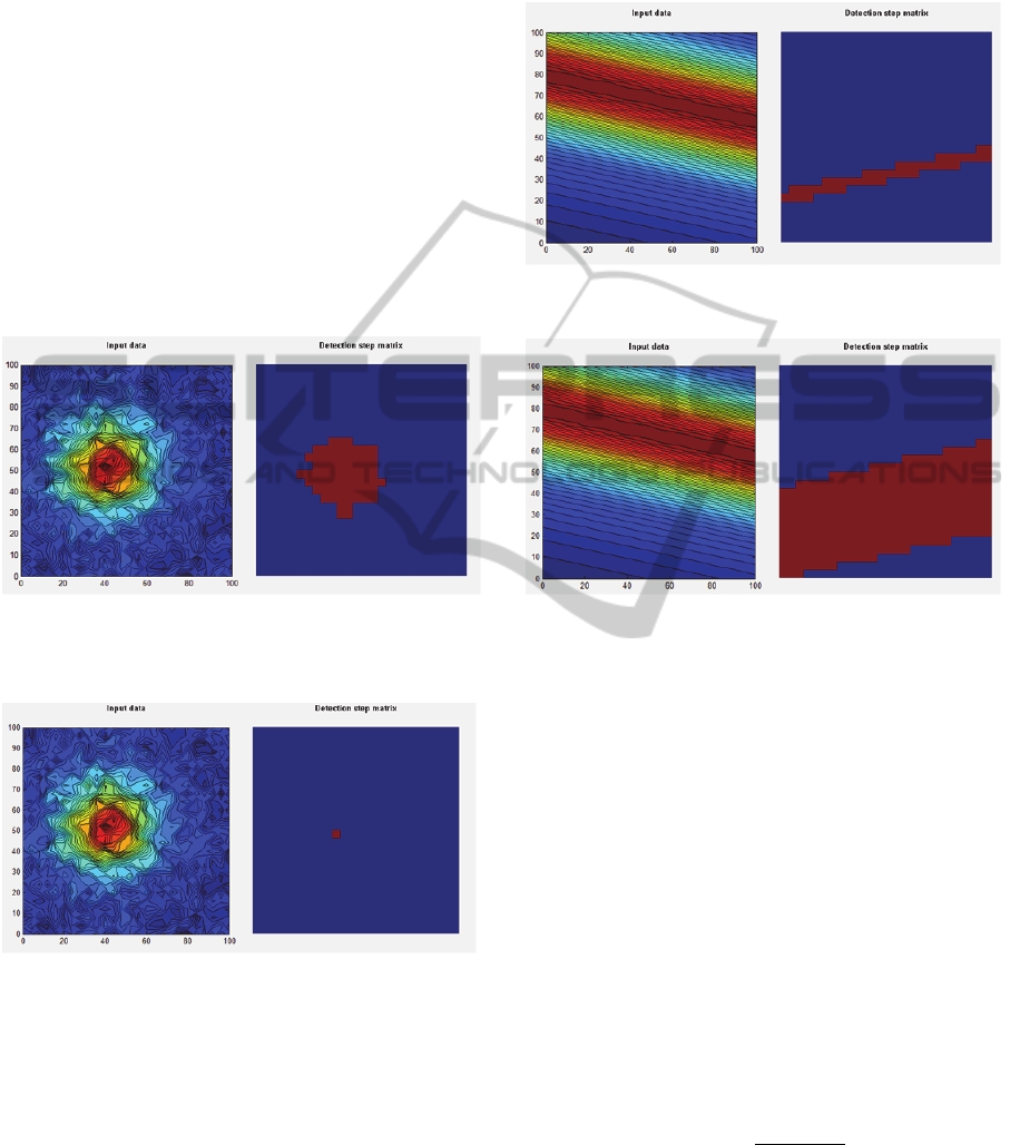
Figure 2: The spherical anomaly with noise (left picture,
noise level is from 0 to 0.2 of the maximum value) and
corresponding HM matrix.
Figure 3: The spherical anomaly with noise (left picture,
noise level is from 0 to 0.2 of the maximum value) and
corresponding MM matrix after erosion.
Next step is the erosion of the MM matrix, as the
erosion pattern is used the Golay alphabet, the L
element (Golay, 1969). The aim of the erosion is
thin the white areas (for a pixel or a single line).
This way we get the location of the middle of the
anomaly.
Now the HM matrix is taken into the account. If
lines were detected, we run the line detection again,
to get the border of the half value area (half middle
line). The distance between the middle line and half
middle line is calculated using standard algebra
algorithms for the line distance measurements.
Figure 4: The horizontal cylinder without noise (left
picture) and corresponding MM matrix after erosion.
Figure 5: The horizontal cylinder without noise (left
picture) and corresponding HM matrix.
If no line is detected, we estimate the width and
height of the white area in HM matrix. If the shape
is not close to the circle, the process ends with result
“no desired anomaly is detected”. Otherwise, the
distance from the middle point to the border of the
half maximum circle is measured.
Measured distance is in the next step used to
estimate the density or mass of the anomaly.
The estimated parameters are used with equation
(1) to calculate the estimated anomaly field. If the
horizontal cylinder was already detected in the data
(the initial line detection was successful), the
process ends.
If no lines were detected, it is now necessary to
distinguish the sphere and vertical cylinder. The
eucleidian distance between the input (
and
estimated (
field is measured point by point for
both estimated anomaly fields and input data:
,
(3)
The result is the distance matrix. The mean value of
this matrix is taken as the error number ErrNum, the
description of the similarity of input and estimated
field. The less is the ErrNum, the closest are values
ApplicationofEdgeandLineDetectiontoDetectthenearSurfaceAnomaliesinPotentialData
695
in the input and estimated field. The estimated shape
of the anomaly is selected as the shape of the
estimated data with lower ErrNum.
3 CONCLUSIONS
The presented shape detection algorithm detects the
analytical anomaly body in both noise-free and noise
data. If low level noise is presented in the data, the
algorithm works well without smoothing the data;
higher level of noise in the data requires the
smoothing.
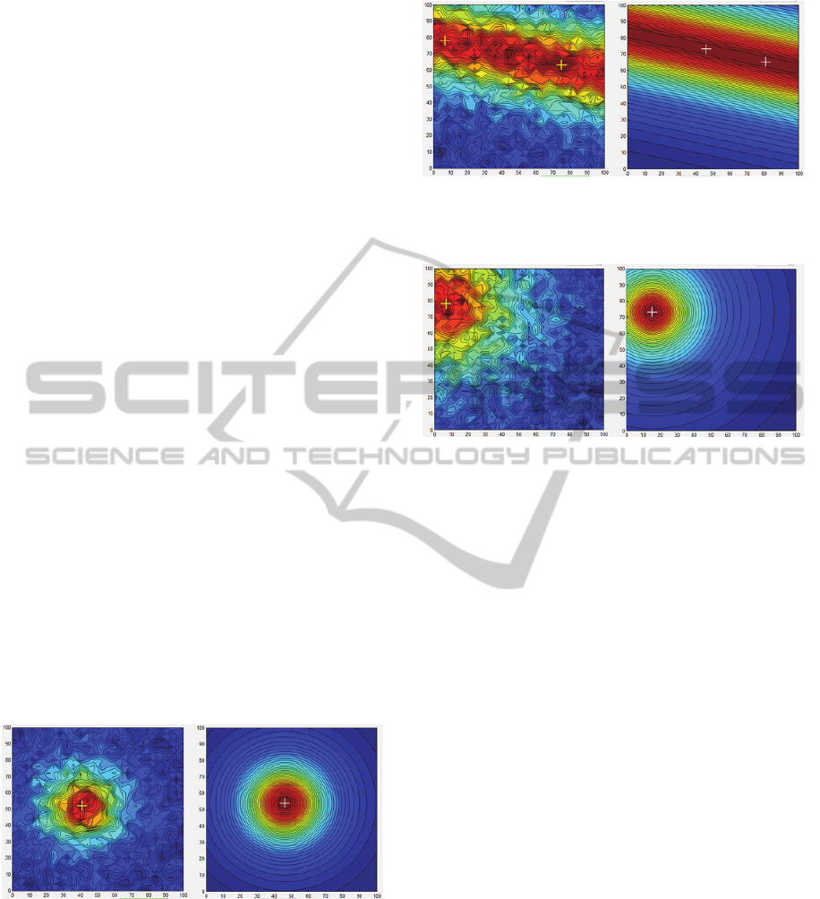
The spherical anomaly detection with high level
of added noise is presented in Figure 6, horizontal
cylinder with the same level of noise in Figure 7,
vertical cylinder is presented in Figure 8. In all
figures, the data area is 100x100 m with 4 m step.
In general, the estimation error differs from 80 %
to 99 % in the depth and location estimation. The
geometry is detected correctly in 80 %. The most of
the failures is obtained with high noise and
horizontal cylinder. For the future we plan to
enhance the shape detection of HM matrix to obtain
the more precise detection and to improve the
comparison of the similarity of the estimated and
input data.
The real application of presented algorithm
requires to define the desired anomaly body and to
modify the proper way the shape detection steps.
If no desired anomaly is presented in data, we
can see it in histogram and also during the shape
detection process (the HM matrix has different than
excepted characteristics).
Figure 6: The spherical anomaly with noise (left picture,
noise level is from 0 to 0.2 of the maximum value) and
estimated value. Original depth is 23 m, estimated is 25 m.
REFERENCES
Aydogan, D., 2012, CNNEDGEPOT: CNN based edge
detection of 2D near surface potential field data,
Computers & Geosciences, vol. 46, p. 1-8.
Figure 7: The horizontal cylinder with noise (left picture,
noise level is from 0 to 0.2 of the maximum value) and
estimated value. Original depth is 22 m, estimated is 23 m.
Figure 8: The vertical cylinder with noise (left picture,
noise level is from 0 to 0.2 of the maximum value) and
estimated value. Original depth is 22 m, estimated is 16 m.
Cooper, G. R. J., 2004, The textural analysis of gravity
data using co-occurrence matrices, Computers &
Geosciences, vol. 30, p. 107-115.
Blakely J. R., 1995, Potential Theory in Gravity &
Magnetic Applications, Cambridge University Press.
Cambridge.
Golay, M. J. E., 1969, Hexagonal Parallel Pattern
Transformations, IEEE Transactions on Computers,
vol. 8, p. 733 – 740.
Li H., Liao X., Li C. et al., 2011, Edge detection of noisy
images based on cellular neural networks,
Communications in Nonlinear Science and Numerical
Simulation, vol. 16, p. 3746-3759.
Mareš S., 1990. Úvod do užité geofyziky, SNTL. Praha, 2
nd
edition.
Matlab, 2009, Image processing toolbox manual,
Mathworks.
Salem A., 2011. Multi-deconvolution analysis of potential
field data, Journal of Applied Geophysic, vol. 74, p.
151-156.
Shih F. Y., 2010. Image processing and pattern
recognition – Fundamentals and Techniques, John
Wiley and Sons. New York.
ICPRAM2013-InternationalConferenceonPatternRecognitionApplicationsandMethods
696
