
Non-local Huber Regularization for Image Denoising
A Hybrid Approach of Two Non-local Regularizations
Suil Son, Deokyoung Kang and Suk I. Yoo
School of Computer Science and Engineering, Seoul National University, Seoul, Republic of Korea
Keywords:
Denoising, Non-local Means, Total Variation Regularization, Non-local Total Variation Regularization,
Non-local H
1
Regularization.
Abstract:
Non-local Huber regularization is proposed for image denoising. This method improves the non-local total
variation regularization and the non-local H
1
regularization approaches. The non-local total variation regular-
ization preserves edges better than the non-local H
1
regularization; however, it leaves a little noise. In contrast,
the non-local H
1
regularization eliminates noise better than the non-local total variation regularization; how-
ever, it blurs edges. To take both advantages of the two methods, the proposed method applies the non-local
total variation to large non-local intensity differences and applies the non-local H
1
regularization to small
non-local intensity differences. A boundary value to determine whether the intensity difference comes from
edges or noise is also suggested. The experimental results of the proposed method is compared to the result
from the non-local total variation regularization and to the result from the non-local H
1
regularization; The
effect of the boundary value is illustrated as PSNR changes with respect to the various values of the boundary
values.
1 INTRODUCTION
Denoising has been consistently studied in the im-
age processing field. As a method to enhancing the
quality of images, it is widely applied to many image
processing applications’ pre-processing step. Since a
good image quality enables the better result of the ap-
plications, the denoising is still active research area.
Smoothing is a primitive denoising method (Lin-
denbaum et al., 1994). A noisy image usually con-
tains large intensity differences between neighbour-
ing pixels; The large differences can be eliminated by
the Gaussian convolution. Therefore, eliminating the
noise of an image, the convolution can reduce the de-
gree of the intensity differences between neighbours.
The convolution however blurs the edge of images.
Though an anisotropic filter can reduce this blurring
effect (Perona and Malik, 1990), such a simple fil-
tering approach still has a difficulty in restoing detail
textures of complex images.
Defining denoising as optimization of a signal,
approaches reconstructing the signal have been pro-
posed. Under this formulation, the Tikhonov regu-
larization (Tikhonov and Arsenin, 1977) and Wiener
filter(Yaroslavsky, 1985) method have been solutions
to the signal reconstruction problem. Rudin, Osher,
and Fatemi also proposed the total variation mini-
mization (Rudin et al., 1992) having good properties
such as preserving edges while eliminating noises.
This method has been widley extended in many re-
searches (Chambolle, 2004; Osher et al., 2003; Osher
et al., 2005; Marquina, 2009).
Transforming an image into another domain and
analyzing it have been also suggested. Fourier trans-
form, discrete cosine transform, and the wavelet
transform are the methods (Yaroslavsky, 1996;
Donoho and Johnstone, 1995; Donoho, 1995; Tem-
izel and Vlachos, 2005). Applied by these meth-
ods, various components in an image can be separated
in the transformed domain. Based on this property,
the noise component was selectively eliminated, and
the denoised images were reconstructed by an inverse
transform from the remained components. The trans-
form approaches however have distorted images re-
sulting in some artifacts.
Statistical approaches have been also applied to
denoising problems. Assuming that a distribution of
noise obeys a zero mean Gaussian distribution, noise
can be successfully eliminated by taking a statistical
mean image if there are several images for a single
scene. Even though given just a single image, the sta-
tistical approach can be still applicable using small
554
Son S., Kang D. and I. Yoo S. (2013).
Non-local Huber Regularization for Image Denoising - A Hybrid Approach of Two Non-local Regularizations.
In Proceedings of the 2nd International Conference on Pattern Recognition Applications and Methods, pages 554-559
DOI: 10.5220/0004263705540559
Copyright
c
SciTePress

image patches located at several parts of the image.
Buades et al. have suggested a non-local means al-
gorithm calculating similarity weighted intensity for
each pixel in an image(Buades et al., 2005). To de-
termine an intensity of each pixel in a denoised im-
age, several image patches are selected, weighted by
a similarity between the patch whose center is the
target pixel, and then averaged. Since this method
preserves a detail texture of a patterned image, many
approaches to extend it have been proposed(Buades
et al., 2006; Gilboa and Osher, 2008; Lee et al., 2011).
The non-local means algorithm has been extended
to combine various regularizations in the optimization
filed (Gilboa et al., 2006; Peyre et al., 2008; Lou et al.,
2010). In these works, the non-local total variation
and the non-local H
1
norm are defined to link the tra-
ditional optimization problem and the non-local ap-
proach. The non-local total variation regularization
particularly showed the good restoration of detailed
texture while preserving edges.
In this paper, we propose a more improvement in
non-local regularization. The proposed non-local Hu-
ber regularization is the improvement of the non-local
total variation regularization and the non-local H
1
regularization. Though the non-local total variation
regularization preserves edges, it sometimes leaves
small noise. To completely eliminate this small noise,
the non-local H
1
regularization is better than the non-
local total variation regularization. However, the non-
local H
1
regularization sometime blurs edges com-
pared to the non-local total variation regularization.
Both of the noise and the edge cause intensity differ-
ences between pixels. If the distinction of the cause
between the noise and the edge is possible, the noise
can be eliminated by the non-local H
1
regularization
and the edge can be preserved by the total variation
regularization. Given a boundary value by which the
distinction is possible, the proposed non-local Huber
regularization applies a linear penalty, the non-local
total variation regularization, for larger values than
the boundary and a quadratic penalty, the non-local
H
1
regularization, for smaller values. A guideline to
selecting the boundary value between the linear and
the quadratic regularization is also suggested.
The remainder of this paper is organized as fol-
lows: The related denoising approeaches are intro-
duced in Section 2, and our non-local Huber regular-
ization approach is explained in Section 3. Specif-
ically, the non-local Huber regularization is formu-
lated in Section 3.1, and the method to the bound-
ary selection is suggested in Section 3.2. The ex-
perimental results in Section 4 demonstrate that our
approach improves existing non-local denoising ap-
proaches. Finally, we conclude in Section 5.
2 NON-LOCAL
REGULARIZATIONS
Given Ω ⊂ R
2
, let u ∈ Ω → R be an original image,
and let o ∈ Ω → R be an observed image for the image
u as follows:
o = K u + n (1)
where K is a linear operator representing image trans-
formation, and the n is a white Gaussian noise. Then,
the denoising is a process obtaining the u from the o.
In the regularized optimization formulation, the
denoised image can be obtained from following equa-
tion
u = arg min
u
1
2
||o − K u||
2
+ λJ(u), (2)
where ||·|| is the l
2
norm, J is a regularization applied
to the u, and λ > 0 is a Lagrange multiplier.
Under the formulation of the equation (2), J is
called as several names depending on its configura-
tion. Among the configurations, the total variation is
defined as
J
TV
(u) =
Z
Ω
|∇u(x)|dx (3)
(Rudin et al., 1992).
Non-local means algorithm defines a new inten-
sity of pixel x as a weighted average of intensities
from non-local pixels, using a function w
o
(Buades
et al., 2005):
NL
o
(x) =
1
C(x)
Z
Ω
w
o
(x,y)o(y)dy, (4)
where the C is a normalization function, and the w
o
is
a similarity function defined as
w
o
(x,y) = exp
− d
a
(o(x),o(y))
(5)
. The function d
a
computes a distance between two
image patches like
d
a
(o(x),o(y)) =
Z
Ω
G
a
(t)|o(x +t)−u(y+t)|
2
dt (6)
where the G
a
is a Gaussian function whose standard
deviation is a. C in the equation (4) is defined as
C(x) =
Z
Ω
w
o
(x,y)dy (7)
Using the equation (4), a non-local mean image
can be obtained by applying the non-local regulariza-
tion,
J
NLM
(u) =
Z
Ω
(u(x) − NL
o
(x))
2
dx (8)
, into the equation (2) (Buades et al., 2005).
Non-local total variation was suggested to com-
bine the non-local means approach and the total vari-
ation approach. In this approach, the non-local gra-
dient ∇
w
u : Ω → Ω × Ω and the non-local divergence
Non-localHuberRegularizationforImageDenoising-AHybridApproachofTwoNon-localRegularizations
555

div
w
−→
v : Ω × Ω → Ω are defined (Gilboa and Osher,
2008):
(∇
w
u)(x,y) := (u(y) −u(x))
p
w(x,y), x, y ∈ Ω (9)
(div
w
−→
v )(x) :=
Z
Ω
(v(x,y) − v(y,x))
p
w(x,y)dy
(10)
Using these non-local operator, non-local regulariza-
tions are defined (Lou et al., 2010; Gilboa and Osher,
2008) as
J
NL/TV
(u) =
Z
Ω
|∇
w
u(x)|dx
=
Z
Ω
r
Z
Ω
(u(x) − u(y))
2
w(x,y)dydx
(11)
J
NL/H
1
(u) =
1
4
Z
Ω
|∇
w
u(x)|
2
dx
=
Z
Ω
Z
Ω
(u(x) − u(y))
2
w(x,y)dydx
(12)
where the equation (11) is called as a non-local to-
tal variation regularization, and the equation (12) is
called as a non-local H
1
regularization. These regu-
larizations are a non-local linear regularization and a
non-local quadratic regularization respectively.
3 THE PROPOSED METHOD
3.1 Non-local Huber Regularization
The Huber function is a combination of two functions:
φ
HU B
(x) =
n
M(2|x| −M), |x| > M
x
2
, |x| ≤ M
(13)
This function computes a linear equation for x larger
than a boundary value M and a quadratic equation for
smaller values.
Similarly, the non-local Huber regularization can
be defined using the non-local linear and quadratic
regularizations in (11) and (12). We define the non-
local Huber regularization as
J
HU B
(u) =
Z
Ω
|∇
w
u(x)|
T (x)
·
|∇
w
u(x)|
2
(1−T (x))
dx
(14)
where the T is a threshold function given as
T (x) =
n
1, |∇
w
u(x)| > B(x)
0, |∇
w
u(x)| ≤ B(x)
(15)
Where the value of the function B(x) determines
whether the non-local intensity difference at pixel x
is caused by noise or edge. When the difference is
larger than the value of the B(x), its cause is deter-
mined as the edge, and smaller than or equal to the
value of the B(x), it is determined as the noise. From
this process, the difference from edges is applied to
the linear penalty, the non-local total variation regu-
larization, and the difference from noise is applied to
the quadratic penalty, the non-local H
1
regularization.
3.2 Non-local Huber Boundary
Selection
Assuming that intensity differences caused by edge
are larger than the difference by noise, the value of
B(x) should be smaller than the difference by edge
and be larger than the difference by noise. This con-
figuration enables that the linear penalty is applied to
the edge and the quadratic penalty is applied to the
noisy area.
If the noise level is known, B(x) can be defined by
the noise level for each pixel x.
B(x) = N
o
(x) (16)
However, the noise level of an image is not known in
most cases. For simplicity, consider an image I hav-
ing a uniform intensity for all pixels, and the image
ˆ
I
obtained from the image I by adding zero mean white
Gaussian noise. Then, the noise level of the image
ˆ
I
is proportional to the standard deviation of intensities
of the image.
N
ˆ
I
(x) ∝ σ
ˆ
I
(17)
In addition, the noise level of each pixel may be
different from each other. In this case, it has a follow-
ing relationship:
N
ˆ
I
(x) ∝ 1 −
R
Ω
w
ˆ
I
(x,y)dy
H
ˆ
I
×W
ˆ
I
(18)
The second term in the equation (18) represents the
average similarity of a pixel x between other pixels.
Because of the zero mean white Gaussian noise as-
sumption, pixels with small noise are more than ones
with large noise, and they have larger similarities to
other pixels. Therefore, if a pixel has a large average
similarity to other pixels, it has a small noise level. On
the other hand, if a pixel has a small average similar-
ity, it has a large noise level. Because the maximum
value of the w
ˆ
I
(x,y) is one, the maximum value of the
R
Ω
w
ˆ
I
(x,y)dy is equal to the area of the image. There-
fore, the second term is smaller than or equal to one,
and the whole term is proportional to the noise level
of a pixel x.
Furthermore, consider the noise level in the case
where the w
ˆ
I
(x,y) has its maximum value. In this
case, the pixel x has no difference in intensity to all
of other pixels. This means that its noise level is zero.
ICPRAM2013-InternationalConferenceonPatternRecognitionApplicationsandMethods
556

On the other hand, in the case where the w
ˆ
I
(x,y) has
its minimum value, the average similarity is zero, and
the noise level of a pixel can be obtained only by the
entire image’s noise level. Therefore, combining the
equation (17) and the equation (18), the noise level
for each pixel x is computed as
N
ˆ
I
(x) = σ
ˆ
I
·
1 −
R
Ω
w
ˆ
I
(x,y)dy
H
ˆ
I
×W
ˆ
I
(19)
Most of images do not have a uniform intensity.
The standard deviation of intensities for an image o
having non-uniform intensity is represented by the
sum of the each standard deviation caused by the orig-
inal intensity changes and noise.
σ
o
= σ
original
o
+ σ
noise
o
(20)
σ
noise
o
= σ
o
− σ
original
o
= η · σ
o
,
where η =
σ
o
− σ
original
o
σ
o
(21)
The σ
original
o
is zero for a uniform intensity image; it
is larger than zero for a non-uniform intensity image;
and it is smaller than or equal to the σ
o
for any kind
of image. Therefore, the η is 0 ≤ η ≤ 1. This value
is close to one when the original image has more uni-
formity in its intensity and is close to zero when the
image has large intensity differences. Reflecting these
properties, we suggest a guide-line to the value of
B(x):
B(x) = N
o
(x) = σ
noise
o
·
1 −
R
Ω
w
o
(x,y)dy
H
o
×W
o
= η · σ
o
·
1 −
R
Ω
w
o
(x,y)dy
H
o
×W
o
(22)
4 EXPERIMENTAL RESULTS
In this section, the results of denoising for four classes
of images added with a zero mean white Gaussian
noise are illustrated. The image patch size is 3 × 3,
and the non-local similarity is computed in the 21 ×
21 window range to reduce the computation time.
The results of denoising for each image are shown
in figure 1 to figure 4. In each figure, the result of the
proposed non-local Huber regularization is compared
to the results of the non-local total variation regular-
ization and to the results of the non-local H
1
regular-
ization.
Figure 1(a) is an original airplane image of 128 ×
128, and the figure 1(b) is the noisy image obtained
from the figure 1(a) adding Gaussian noise of stan-
dard deviation 20. Figure 1(c), 1(d), and 1(e) are de-
noised images obtained from the non-local H
1
regu-
larization, the non-local Huber regularization, and the
Table 1: PSNRs of the denoised images from Figure 1, 2, 3,
and 4.
images NLH
1
NLHUB NLTV
airplane 22.80 23.52 19.93
barba 20.76 24.08 22.92
boat 21.82 21.31 20.29
lenna 21.10 22.03 20.70
non-local total variation regularization, respectively.
Similarly, figure 2(a), 3(a), and 4(a) are original im-
ages, and their noised images using the same Gaus-
sian noise to previous one are shown in figure 2(b),
3(b), and 4(b). Figure 2(c), 3(c), and 4(c) are their
denoised images obtraind from the non-local H
1
reg-
ularization, Figure 2(d), 3(d), and 4(d) are from the
non-local Huber regularization, and Figure 2(e), 3(e),
and 4(e) are from the non-local total variation regular-
ization. All of the denoising above have used η = 0.1.
As shown in the results, the non-local H
1
regu-
larization results in blurry denoised images, and the
non-local total variation regularization gives clearer
results than the result of the non-local H
1
regulariza-
tion. Compared to the results from other approaches,
the proposed non-local Huber regularization gives a
similar result to the one of the non-local total variation
regularization. Particularly, for figure 1, the non-local
Huber regularization gives clearer result than the one
from the non-local total variation regularization.
The peak signal to noise ratio (PSNR) results of
the figure 1, 2, 3, and 4 are shown in the table 1. As
shown in the table, except the boat image, the PSNRs
from the non-local Huber regularization show the
highest values compared to other approaches. Though
the non-local H
1
regularization shows the highest
PSNR for the boat image, The non-local Huber reg-
ularization is better at visualizing the denoised image
than the non-local H
1
regularization.
Using various values for η, the PSNR changes
of the images from the non-local Huber regulariza-
tion are shown in the figure 5. Figure 5(a) shows the
denoised results for the noisy images obtained from
the images in the figure 1(a), 2(a), 3(a), and 4(a) by
adding a zero mean white Gaussian noise whose stan-
dard deviation is 10, and the figure 5(b) shows the de-
noised results for the same images with noise whose
standard deviation is 20. As shown in the figure 5, the
PSNR with η ≤ 0.1 is larger than the one with η = 0,
and the highest PSNR results around η = 0.1. Since
the non-local Huber regularization with η = 0 is equal
to the non-local total variation regularization, the non-
local Huber regularization shows better PSNR than
non-local total variation regularization for η ≤ 0.1.
Non-localHuberRegularizationforImageDenoising-AHybridApproachofTwoNon-localRegularizations
557
(a) (b) (c) (d) (e)
Figure 1: Airplane images with 128 × 128 size. 1(a) is an original image. 1(b) is an image with noise of standard deviation 20
from the original image. 1(c) is a result from the non-local H
1
regularization. 1(d) is from the non-local Huber regularization.
1(e) is from the non-local total variation regularization.
(a) (b) (c) (d) (e)
Figure 2: Barba images with 128 × 128 2(a) is an original image. 2(b) is an image with noise of standard deviation of 20 from
the original image. 2(c) is a result from non-local H
1
regularization. 2(d) is from non-local Huber regularization. 2(e) is from
non-local total variation regularization.
(a) (b) (c) (d) (e)
Figure 3: Boat images with 128 × 128 3(a) is an original image. 3(b) is an image with noise of standard deviation of 20 from
the original image. 3(c) is a result from the non-local H
1
regularization. 3(d) is from the non-local Huber regularization. 3(e)
is from the non-local total variation regularization.
(a) (b) (c) (d) (e)
Figure 4: Lenna images with 128 × 128 4(a) is an original image. 4(b) is an image with noise of standard deviation of 20 from
the original image. 4(c) is from the non-local H
1
regularization. 4(d) is from the non-local Huber regularization. 4(e) is from
the non-local total variation regularization.
5 CONCLUSIONS
In this paper, we have proposed the non-local Huber
regularization enhancing the non-local total variation
regularization for image denoising. This method ap-
plied the non-local total variation and the non-local
H
1
regularization depending on the degree of the non-
ICPRAM2013-InternationalConferenceonPatternRecognitionApplicationsandMethods
558
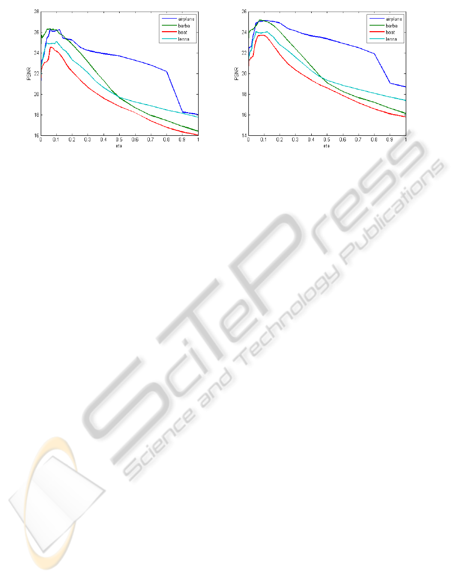
(a) (b)
Figure 5: PSNR plot of denoised images for various η values. 5(a) is results from images with noise of standard deviation of
10 from the original images. 5(b) is results from images with noise of standard deivation of 20 from the original images.
local intensity differences based on a boundary value.
To properly apply this method, selection of the bound-
ary value was also suggested. Using the proposed
method, higher PSNR results and clearer denoised
images were obtained compared to the results from
the non-local total variation regularization and to the
results from the non-local H
1
regularization.
REFERENCES
Buades, A., Coll, B., and Morel, J.-M. (2005). A non-local
algorithm for image denoising. IEEE Preceedings of
Computer Vision and Pattern Recognition.
Buades, A., Coll, B., and Morel, J. M. (2006). Image en-
hancement by non-local reverse heat equation. Tech-
nical Report.
Chambolle, A. (2004). An algorithm for total variation min-
imization and applications. Journal of Mathematical
Imaging and Vision, pages 89–97.
Donoho, D. L. (1995). De-noising by soft-thresholding.
IEEE Transaction on Information Theory, 41:612–
627.
Donoho, D. L. and Johnstone, I. M. (1995). Adapting to un-
known smoothness via wavelet shrinkage. Journal of
the American Statistical Association, 90:1200–1224.
Gilboa, G., Darbon, J., Osher, S., and Chan, T. (2006).
Nonlocal convex functionals for image regularization.
UCLA CAM Report.
Gilboa, G. and Osher, S. (2008). Nonlocal operators with
applications to image processing. Multiscale Model
and Simulation, 7:1005–1028.
Lee, C., Lee, C., and Kim, C.-S. (2011). Mmse nonlocal
means denoising algorithm for poisson noise removal.
IEEE International Conference on Image Processing.
Lindenbaum, M., Fischer, M., and Bruckstein, A. M.
(1994). On gabor contribution to image enhancement.
Pattern Recognition, pages 1–8.
Lou, Y., Zhang, X., Osher, S., and Bertozzi, A. (2010). Im-
age recovery via nonlocal operators. Journal of Scien-
tific Computing, pages 185–197.
Marquina, A. (2009). Nonlinear inverse scale space meth-
ods for total variation blind deconvolution. Society of
Industrial Applied Mathematics, 2:64–83.
Osher, S., Burger, M., Goldfarb, D., Xu, J., and Yin, W.
(2005). An iterative regularization method for total
variation-based image restoration. Multiscale Model-
ing and Simulation, 4:460–489.
Osher, S., Sole, A., and Vese, L. (2003). Image decomposi-
tion and restoration using total variation minimization
and the h
−1
norm. Society for Industial and Applied
Mathematics, 1:349–370.
Perona, P. and Malik, J. (1990). Scale space and edge de-
tection using anisotropic diffusion. IEEE Transaction
on Pattern Analysis and Machine Intelligence, pages
629–639.
Peyre, G., Bougleux, S., and Cohen, L. (2008). Non-local
regularization of inverse problems. European Confer-
ence on Computer Vision, pages 57–68.
Rudin, L. I., Osher, S., and Fatemi, E. (1992). Nonlinear to-
tal variation based noise removal algorithms. Physica,
pages 259–268.
Temizel, A. and Vlachos, T. (2005). Wavelet domain image
resolution enhancement using cycle-spinning. IEEE
Electronics Letters, 41:119–121.
Tikhonov, A. and Arsenin, V. (1977). Solution of ill-posed
problems. Wiely, New York.
Yaroslavsky, L. (1985). Digital picture processing - an in-
troduction. Springer Verlag.
Yaroslavsky, L. (1996). Local adaptive image restoration
and enhancement with the use of dft and dct in a run-
ning window. Proceedings of Wavelet Applications in
Signal and Image Processing, pages 1–13.
Non-localHuberRegularizationforImageDenoising-AHybridApproachofTwoNon-localRegularizations
559
