
Prediction of Organ Geometry from Demographic and
Anthropometric Data based on Supervised Learning Approach
using Statistical Shape Atlas
Yoshito Otake
1,2
, Catherine Carneal
3
, Blake Lucas
1
, Gaurav Thawait
4
, John Carrino
4
, Brian Corner
5
,
Marina Carboni
5
, Barry DeCristofano
5
, Michale Maffeo
5
, Andrew Merkle
3
and Mehran Armand
2,3
1
Department of Computer Science, The Johns Hopkins University, Baltimore, MD, U.S.A.
2
Department of Mechanical Engineering, The Johns Hopkins University, Baltimore, MD, U.S.A.
3
Applied Physics Laboratory, The Johns Hopkins University, Laurel, MD, U.S.A.
4
Department of Radiology, The Johns Hopkins Hospital, Baltimore, MD, U.S.A.
5
US Army Natick Soldier Research Development and Engineering Center, Natick, MA, U.S.A.
Keywords: Statistical Shape Atlas, Demographic and Anthropometric Data, Principal Component Analysis, Regression
Analysis, Supervised Learning, Allometry.
Abstract: We propose a method relating internal human organ geometries and non-invasively acquired information
such as demographic and anthropometric data. We first apply a dimensionality reduction technique to a
training dataset to represent the organ geometry with low dimensional feature coordinates. Regression
analysis is then used to determine a regression function between feature coordinates and the external
measurements of the subjects. Feature coordinates for the organ of an unknown subject are then predicted
from external measurements using the regression function, subsequently the organ geometry is estimated
from the feature coordinates. As an example case, lung shapes represented as a point distribution model was
analyzed based on demographic (age, gender, race), and several anthropometric measurements (height,
weight, and chest dimensions). The training dataset consisted of 124 topologically consistent lung shapes
created from thoracic CT scans. The prediction error of lung shape of an unknown subject based on 11
demographic and anthropometric information was 10.71 ± 5.48 mm. This proposed approach is applicable
to scenarios where the prediction of internal geometries from external parameters is of interest. Examples
include the use of external measurements as a prior information for image quality improvement in low dose
CT, and optimization of CT scanning protocol.
1 INTRODUCTION
Analysis of organ geometries using statistical shape
atlases is a prevalent trend in various target
application fields, such as cardiac modelling (Frangi
et al., 2002), pelvis shape analysis for dose reduction
(Chintalapani et al., 2010), 4-dimensional lung
motion modelling (Ehrhardt et al., 2011), and a
small animal research using Micro-CT (Hongkai
Wang et al., 2012).
Most existing statistical shape atlases of human
organ are created from an unnonimized CT dataset,
thus the analyses were often confined to organ shape
among a select disease group or subject population.
To our knowledge, the relationship between
anthropometric and demographic data with a
statistical atlas of generalized population is not
investigated as yet.
In order to address this gap, we collected a
thoracic computed tomography (CT) dataset together
with non-invasively acquired “external
measeurements” including demographic information
and several anthropometric metrics. We propose a
method to analyze correlation between a subject’s
external measurements and their internal organ
geometry based on a supervised learning approach.
As an initial feasibility study, we used lung as a
target organ and considered its geometric features as
a cloud of connected points (Point Distribution
Model, PDM).
Prediction of information about internal structure
which are typically measured in invasive way from
these readily measureable external measurements
365
Otake Y., Catherine C., Lucas B., Thawait G., Carrino J., Corner B., Carboni M., DeCristofano B., Maffeo M., Merkle A. and Armand M. (2013).
Prediction of Organ Geometry from Demographic and Anthropometric Data based on Supervised Learning Approach using Statistical Shape Atlas.
In Proceedings of the 2nd International Conference on Pattern Recognition Applications and Methods, pages 365-374
DOI: 10.5220/0004263803650374
Copyright
c
SciTePress
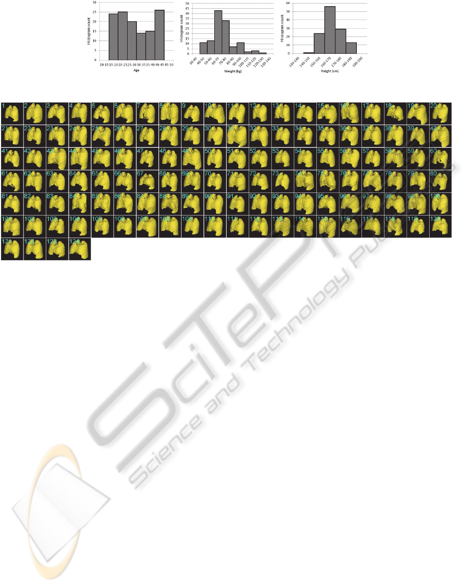
Figure 1: Demographic property distributions of the population in training dataset.
Figure 2: Training dataset. PDM (Point Distribution Model) of lung geometry of 124 subjects were created from CT dataset.
Automatic segmentation combined with a deformable registration algorithm (Mjolnir (Ellingsen, Chintalapani, Taylor, &
Prince, 2010)) using one subject (subject #44) as a template was employed to obtain topology-consistent meshes. Thus
point correspondence was inherently solved. The subjects were chosen in such a way that the demographic characteristics
were well balanced.
may be useful in a variety application scenarios
ranging from medical device development to
personalized medicine and protection. The use of
external measurements as a prior information for
image quality improvement in low dose CT, and
optimization of CT scanning protocol are two
potential example applications for this approach.
2 METHODS
2.1 Materials
Existing radiological CT scans of the chest region
were collected from 124 patients. Following Johns
Hopkins Institutional Review Board (IRB) approval,
the radiology archives at Johns Hopkins Hospital
were searched for thoracic or chest CT scans of
males and females ages 17-45. Only very strictly
normal scans of lung were included in this study
(normal by report and inspection). Any scan with
obvious or minimal pathology was excluded. Scans
that showed lungs without disease but with findings
different from normal (such as atelectasis, normal
variants) were also excluded. Subject characteristics
of age, gender, ethnicity, height and weight were
extracted from their medical records archives. In
order to reduce population bias in the statistical
atlas, the patients were selected to achieve a
relatively even distribution of gender and ethnicity.
For the purpose of this initial study, ethnic groups
were binned as White, Black, Hispanic, and Other.
Subjects were anonymized after extraction. Table 1
and Figure 1 show the distribution of demographic
property of the population in the training dataset.
External measurements of each subject’s chest
span, chest depth, chest breadth, and inter-nipple
distance were manually approximated from
landmarks on the CT images. These measurements
were selected to correspond with those used in
common anthropometric surveys ((Gordon et al.,
1989); (Robinette et. al., 2002)). Chest span (cranio-
caudal) was defined as the vertical distance between
highest level of first rib to the lower costophrenic
angle. Chest breadth (or width) was defined as the
skin to skin depth of the chest at the carinal plane at
the level of nipples. Finally, the inter-nipple distance
measurement was made in an axial plane view
where both nipples were visible.
ICPRAM2013-InternationalConferenceonPatternRecognitionApplicationsandMethods
366
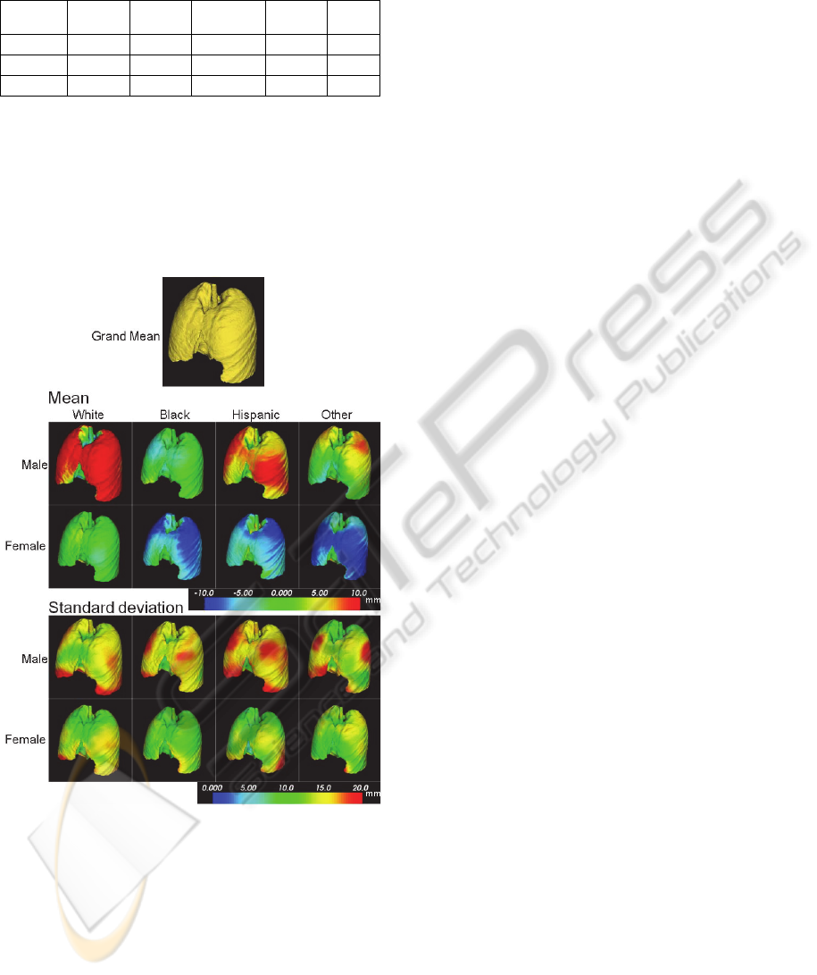
Table 1: Number of subjects in each population group in
the training dataset.
White
(n)
Black
(n)
Hispanic
(n)
Other
(n)
Total
(%)
Male (n)
19 15 14 12 48.4
Female (n)
19 17 14 14 51.6
Total (%)
31.6 25.8 22.6 21.0 100
2.2 Construction of Training Datasets
We selected a template CT image from the acquired
dataset. This template was manually segmented, and
used to generate a template tetrahedral mesh
consisting of 112,602 vertices and 509,034
tetrahedrons.
Figure 3: Mean shape (upper 2 rows) and standard
deviation (lower 2 rows) of the training dataset in each
population group. Colormap of mean indicates the
displacement of each vertex from the grand mean (mean
of the entire population) along the normal direction of a
triangle mesh at each vertex, positive indicating outward
direction.
An intensity based deformable registration
method (Mjolnir, (Ellingsen et al., 2010)) was
applied to deformably register the CT data of each
subject to the template CT. The resulting
deformation field was applied to the template mesh
to create a tetrahedral mesh representing the
particular subject. Thus, the point correspondences,
which is one of the key considerations in a typical
statistical atlas construction process, was inherently
solved in our pipeline.
Figure 2 shows the entire training dataset that we
used in this study. The mean of white male was
more than 10 mm larger than the grand mean, and
the means of female were almost the same (for
White) or about 10 mm smaller than the grand mean.
Figure 3 shows the mean shape and standard
deviation among each population group classified
based on race and gender.
2.3 Proposed Approach
As shown in Figure 4, the workflow of the proposed
method consists of 2 steps including a modelling
step and a prediction step.
In the modelling step, we modelled each shape
instance as a vector of X, Y, Z coordinates of all the
mesh vertices and applied dimensionality reduction
algorithm which creates low dimensional feature
coordinates for each subject. Two types of
dimensionality reduction algorithms were tested,
principal component analysis (PCA) (Figure 5) and
Isomap (Tenenbaum et al., 2000). Linear least
square regression analysis was performed to
compute a regression function between the feature
coordinates (also called mode weights in PCA) and
the external measurements of the subject.
The prediction step predicted the feature
coordinates of an unknown subject from its external
measurements, and subsequently the organ shape
was estimated from the predicted feature
coordinates. As is the case with a typical regression
analysis, the approach makes it possible to analyze
magnitude and direction of correlation between each
external measurement and the feature coordinates
which encode the organ shape.
The proposed approach makes the analysis of the
complex variation of organ shapes represented as a
large dimensional vector tractable by using
dimensionality reduction. The regression step can
employ more general classes of non-linear
regression methods, although a simple linear least
square approach was used in our feasibility study
reported here.
The following subsections detail each step in the
proposed workflow.
2.3.1 Dimensionality Reduction
An organ geometry was represented as a 3V-vector
PredictionofOrganGeometryfromDemographicandAnthropometricDatabasedonSupervisedLearningApproachusing
StatisticalShapeAtlas
367
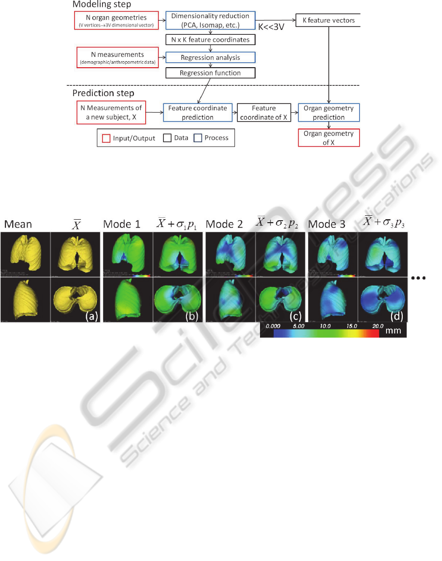
Figure 4: Overview of the workflow of organ geometry prediction. Modelling step reduces dimensionality of the organ
geometry based on the training dataset and produces feature vectors and feature coordinates of each geometry. Then a
regression function was created by a regression analysis on the demographic/anthropometric data and the feature
coordinates. Prediction step determines shape of the target organ of a new subject based on feature coordinates predicted by
the regression function.
Figure 5: PCA analysis on point distribution model of lungs of the training dataset. (a) mean shape, mean plus one standard
deviation in the direction of mode 1 (b), mode 2 (c), and mode 3 (d). The colormap (0-20 mm) shows displacement of each
vertex from the mean shape.
x
i
, (V: number of vertices, i: index of the subject).
Principal Component Analysis. PCA was
performed on the set
,,…,
(N: number
of subjects) creating a new feature coordinate system
that represents each geometry
1
(1)
where e
j
represents the feature vectors (principal
mode vectors), which is eigenvectors of the
covariance matrix of x
i
sorted according to ecreasing
eigenvalues
j
. ̅ is the mean shape and a
i
j
are the
feature coordinates (mode weights) that correspond
to each feature vector. M is the number of feature
vectors.
Given a set of feature coordinates for an
unknown subject
,1,…,, its organ
geometry x
u
is estimated (reconstructed) by (1).
Isomap. Isomap is a type of non-linear
dimensionality reduction method where the training
datasets were modelled as weighted graph based on
its distance matrix which produces a new distance
measure called geodesic distance, and then classical
eigen analysis, multidimensional scaling (MDS,
(Borg and Groenen, 2005)) is applied on the
geodesic distances. The connectivity of each data
point in the neighbourhood graph is defined as its k-
Nearest Neighbours (kNN) in the high-dimensional
space. In this paper, a simple Euclidean distance was
used as the distance metric in the high-dimensional
space and K=6 was chosen for kNN. Thus, Isomap
produces feature coordinates
,1,…, for
each subject i from the set of organ geometries
,1,…,
similar to PCA.
For reconstruction of an organ geometry of an
unknown subject x
u
from its feature coordinates, we
used kNN interpolation in the feature space.
ICPRAM2013-InternationalConferenceonPatternRecognitionApplicationsandMethods
368

Figure 6: Distribution of mode weights in the training dataset. Histograms of the first 8 principal modes were plotted.
kNN was computed based on Euclidean distance
between the feature coordinates and an inverse
distance was used as the weight (Shepard, 1968) as
follows.
∑
∈
(2)
where d
i
is the Euclidean distance between two M
dimensional vector a
u
and a
j
. We employed a simple
interpolation scheme due to limitation of
computation time in our initial implementation,
however, a more computationally intensive
interpolation method such as radial basis function
(RBF) (Press, 2007) can also be applied in this step.
2.3.2 Linear Least Square Regression on
Mode Weights and Measurements
Linear least square regression analysis on the feature
coordinates (a
i
j
) and external measurements
,1,…,
were performed. Here X
i
represents
a K-vector consisting of K measurements of i
th
subject.
Using X
i
as independent variables and a
i
j
as an
dependent variable, we computed regression
coefficients A
m
(intercept) and B
m,k
for each feature
coordinate independently. Thus the computed
regression function can be written as follows.
1
1
1,
1
.1
2
2
2,
1
.2
⋮
,
1
.
(3)
2.3.3 Prediction of Organ Geometry from
External Measurements
To compute the organ geometry of an unknown
subject x
u
from a set of external measurement of the
subject X
u
, we first computed a set of its feature
coordinates
,1,…, using the regression
function (3). Then the organ geometry was
computed based on the feature coordinates as
described in 2.2.1.1 and 2.2.1.2 for PCA and Isomap
respectively.
2.4 Validation Method
In order to evaluate accuracy of the proposed
method, leave-out validation tests were performed.
In the first set of tests, 2 subjects (#33 & #47)
were left out. The proposed modelling step was
applied to the training dataset excluding the 2
subjects. Organ geometry of the 2 left-out subjects
were predicted using the proposed approach and
compared with the true geometry. Distance between
the vertices of the predicted and the true shape were
computed as an error metric and colormapped on the
predicted shape.
The second validation tests were a series of
leave-one-out test. 1Each subject was left-out one to
the other, and the same test described above was
repeated.
3 RESULTS & DISCUSSION
3.1 Comparison between Two
Dimensionality Reduction
Algorithms
Figure 7 shows an example sorting of the training
datasets based on the first 2 principal modes (feature
vectors) using the 2 different dimensionality
reduction methods. Subjects in the training datasets
PredictionofOrganGeometryfromDemographicandAnthropometricDatabasedonSupervisedLearningApproachusing
StatisticalShapeAtlas
369
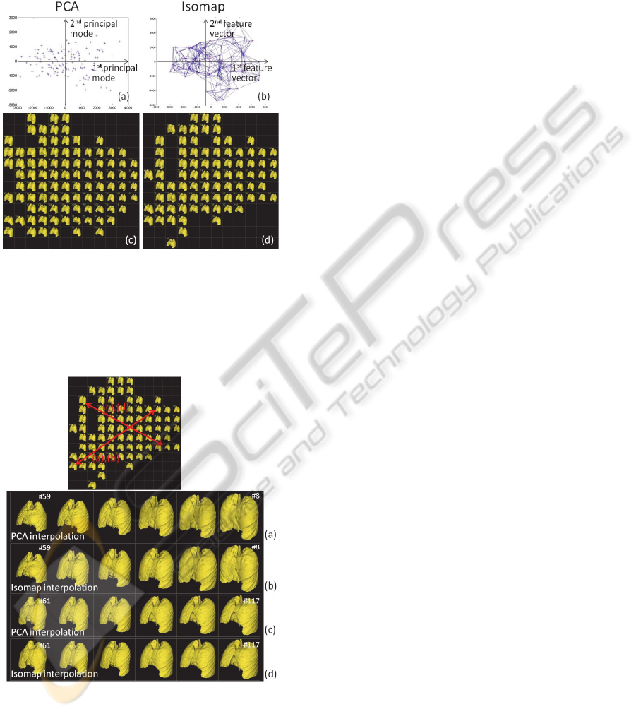
were sorted according to their feature coordinates
and plotted in Figure 7(a) and 7(b). Figure 7 (c) and
7(d) demonstrate lung shapes each corresponding to
the plots above (lung shapes close to each other are
not shown).
Figure 7: A comparison between 2 different
dimensionality reduction algorithms: PCA and Isomap.
The training datasets were sorted based on the first 2
principal modes (feature vectors). (a)(b) plots showing
distribution of the training dataset, (c)(d) lung shape of
each dataset that corresponds to the points in (a)(b). PCA
and Isomap produced very similar results.
Figure 8: A comparison of interpolation using 2 methods.
Interpolation from subject #59 to #8 using (a) Isomap and
(b) PCA, from subject #61 to #117 using (c) Isomap and
(d) PCA. Interpolated geometries were computed by k-NN
interpolation (K=6) of feature coordinates (mode weights)
of the two subjects. Similar to the sorting result (Figure 4),
PCA and Isomap produced very similar results.
Figure 8 shows an example of interpolation
between 2 subjects in the feature space using the 2
different methods. The interpolations were
performed in its feature coordinates and 4
sequentially interpolated shapes (20, 40, 60, 80%
between the two shapes) were shown.
As previous work noted (Seshamani et al., 2011),
PCA and Isomap produced very similar results,
which suggested that the modelling
(parameterization) based on PDM does not produce
a highly nonlinear manifold. However, as shown in
(Tenenbaum et al., 2000), a different type of input
dataset, such as face images, creates nonlinear
manifold which can only captured by nonlinear
dimensionality reduction methods. We believe that
this suggests that the nonlinear algorithm would be
required when CT data itself were used as an input
training dataset rather than PDM. Since the PCA and
Since Isomap produced similar results in the
following discussions, we focus on PCA only.
However, it is notable that any type of linear- or
nonlinear- dimensionality reduction technique can
be used with the proposed method.
3.2 Principal Component Analysis on
the Training Datasets
Figure 8 shows distribution of mode weight values
(a
i
j
) for mode 1 to 8 computed from PCA on the
training datasets. The mode weights nearly followed
normal distribution. Absolute value of the mode
weights indicates the average displacement (mm) of
all the vertices along each mode vector.
3.3 Regression on Mode Weights and
Measurements
Results of the linear least square analysis on the first
10 mode weights were shown in Figure 9. Strong
correlation between mode 1 and a few
anthropometric data (chest breadth, chest span,
height, etc.) was observed. Chest depth and span
also showed higher correlation. From the three plots
Figure 9 a-c), the stronger correlation between mode
1 and height (a), chest breadth (c) than IN distance
(b) were clearly observed.
3.4 Leave-out Validation Test
Two subjects (#33 and #47) were left out, and PCA
and regression analysis were performed using the
other 123 subjects. The accuracy of the prediction of
each mode weight was validated using the left-out 2
subjects. Table 2 shows the error in prediction of the
ICPRAM2013-InternationalConferenceonPatternRecognitionApplicationsandMethods
370
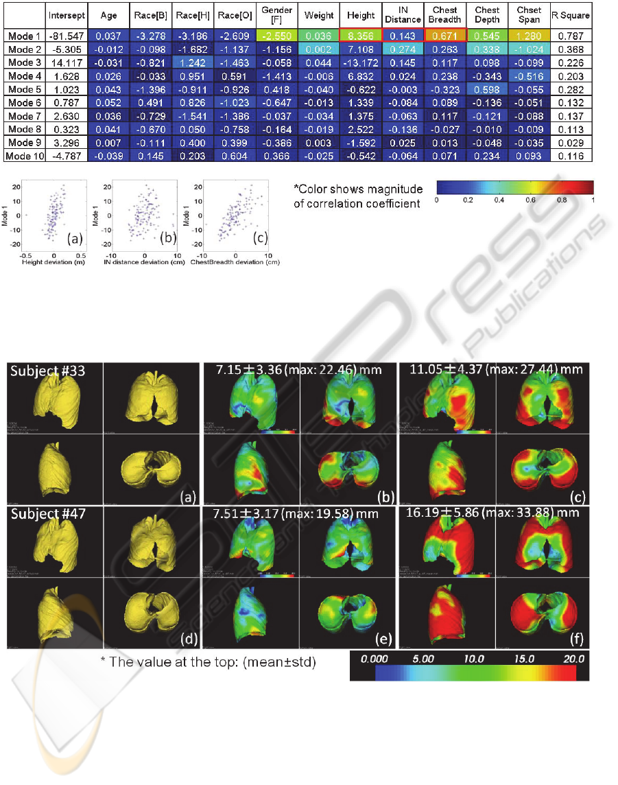
Figure 9: Results of linear least square analysis on the first 10 mode weights and 11 demographic/anthropometric
measurements. The table shows coefficient of the computed regression functions. Magnitude of correlation coefficient was
colormapped in the table. Strong correlation between mode 1 and a few anthropometric data is observed. Chest depth and
chest span showed higher correlation with mode 4 and 5. Distribution of the of representative measurements (height, IN
distance, chest breadth) vs 1st mode weight were shown below left (a)-(c).
Figure 10: Results of the left-two validation test. (a-c) prediction of subject #33 (43 y.o., female, 48.53 kg, 152 cm). (a) true
shape, (b) predicted shape, (c) mean shape. (d-f) true, predicted and mean shape of subject #47 (44 y.o, female, 49.9 kg, 160
cm). The color map shows the error at each vertex from the true shape. The predicted geometries were produced based on
the predicted mode weights using kNN interpolation (K=6) in the feature space.
mode weights. Despite the large variation in the true
mode weights (column 2 and 3), the proposed
method predicted the mode weight with about 2 mm
error on average.
Figure 10 shows the result of prediction of the
lung geometry. We compared our prediction result
(middle column) to the mean shape (right column),
since the mean shape is the best prediction when no
additional information (external measurements) was
involved. Compared to the error distribution in mean
shape, our prediction clearly showed better results in
both subjects especially around the lower edge.
PredictionofOrganGeometryfromDemographicandAnthropometricDatabasedonSupervisedLearningApproachusing
StatisticalShapeAtlas
371
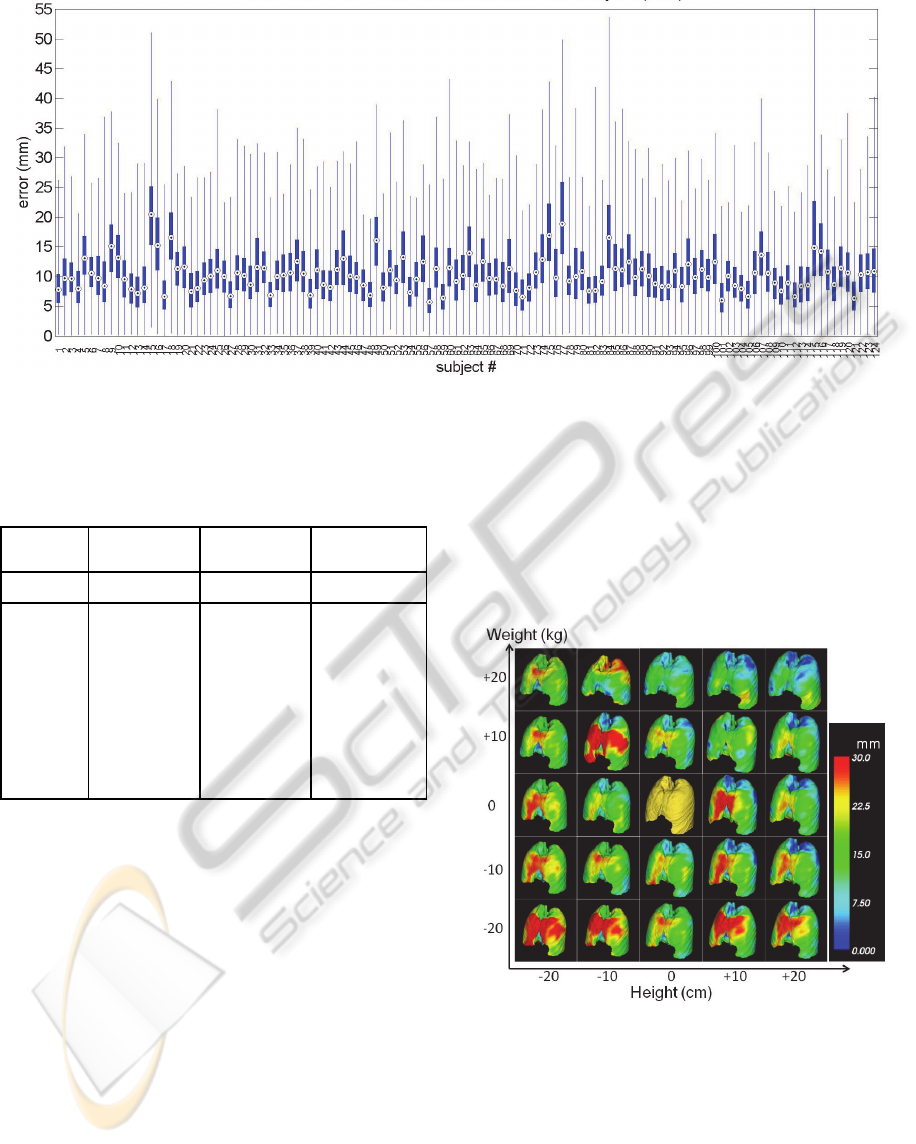
Figure 11: Results of leave-one-out validation test. All 125 subjects were left out and validated one at a time. Each plot
shows the displacement error (mm) at 112,602 vertices of the lung (box plot: 25-75%, whisker plot: maximum and
minimum, dot: median). Mean and standard deviation of the error over the entire subjects were 10.71 ± 5.48 mm.
Table 2: Results of mode weight prediction in leave-two-
out validation test.
True mode
weights (mm)
Predicted mode
weights (mm)
Prediction error
(mm)
Subject ID #33 #47 #33 #47 #33 #47
Mode 1 -8.54 -15.5 -6.68 -11.36 1.85 4.14
Mode 2 -4.10 1.78 -3.80 1.16 0.30 -0.62
Mode 3 -1.56 -0.16 -0.11 -1.50 1.46 -1.34
Mode 4 1.54 -2.10 -0.81 0.51 -2.35 2.61
Mode 5 -1.40 1.83 0.84 3.08 2.24 1.24
Mode 6 -2.28 -0.09 0.75 -0.95 3.03 -0.87
Mode 7 2.34 -2.03 1.10 0.14 -1.25 2.17
Mode 8 0.56 -0.69 0.78 0.07 0.22 0.76
Mode 9 -1.23 -1.39 0.18 0.40 1.41 1.79
Mode 10 -0.61 -0.08 -0.38 -0.53 0.23 -0.45
Results of the repeated leave-one-out validation
tests were shown in Figure 11. The distance error
was about 10 mm on average. A few outliers that
showed much larger error such as #15 or #115 were
attributed as the error in the modelling step due to
either segmentation/registration error.
Figure 12 shows a simple application example of
the proposed workflow where the lung shape was
predicted based on 2 simple external measurements,
height and weight.
4 CONCLUSIONS
We proposed a framework to combine non-
invasively measurable information (demographic/
anthropometric information) with statistical shape
atlas of internal organs using a supervised learning
approach. By incorporating dimensionality reduction
methods, the proposed method can perform
regression analysis with a reasonably small number
of variables which leads the analysis of correlation
between complex shape variation and demographic
information tractable.
Figure 12: An example of lung shape prediction based on
2 demographic parameters (height and weight) using
Isomap. Feature vectors were extracted from 124 training
datasets using Isomap. Regression function was computed
to predict feature coordinate of a new instance based on
the 2 demographic parameters. The figures show lung
shapes when height and weight were varied [-20 +20] cm,
[-20 +20] kg respectively from a typical subject (#36,
68.03 kg, 173 cm). Color map indicates distance at each
vertex from the subject’s lung (shown at the center).
ICPRAM2013-InternationalConferenceonPatternRecognitionApplicationsandMethods
372

The proposed method was piloted on an initial dataset of 124 subjects. Improvement of the
predictive models would likely be achieved by
enlarging the training dataset. Future work includes
sample size analysis to determine the sufficient
number of samples for a particular application.
Additionally, although only four external
anthropometric features were selected in this paper,
improvement of the predictive models may be
increased by increasing the number of external
features employed.
The proposed supervised learning based
workflow consisting of dimensionality reduction and
regression analysis is more broadly applicable to
various cases. For example, CT data itself can be an
input objects rather than PDM.
ACKNOWLEDGEMENTS
This research was supported in part by the United
States Army Natick Soldier Research Development
and Engineering Center. Cleared for public release,
NSRDEC #U12-424.
REFERENCES
Borg, I., & Groenen, P. J. F. (2005). Modern
multidimensional scaling,: Theory and applications
(2nd ed.). New York: Springer.
Gordon, C. C., Churchill, T., Clauser, C. E., Bradtmiller,
B., McConville, J. T., Tebbetts, I., Walker, R. A.
(1989). 1988 Anthropometric Survey of US Army
Personnel: Methods and Summary Statistic. Technical
Report NATICK/TR-89/044, United States Army
Natick Research, Development and Engineering
Center, Natick, MA, USA.
Chintalapani, G., Murphy, R., Armiger, R. S., Lepisto, J.,
Otake, Y., Sugano, N., et al. (2010). Statistical atlas
based extrapolation of CT data. Medical Imaging
2010: Visualization, Image-Guided Procedures, and
Modeling, 7625(1), 762539.
Ehrhardt, J., Werner, R., Schmidt-Richberg, A., &
Handels, H., (2011). Statistical modeling of 4D
respiratory lung motion using diffeomorphic image
registration. Medical Imaging, IEEE Transactions on,
30(2), 251-265.
Ellingsen, L. M., Chintalapani, G., Taylor, R. H., & Prince,
J. L., (2010). Robust deformable image registration
using prior shape information for atlas to patient
registration. Computerized Medical Imaging and
Graphics, 34(1), 79-90.
Frangi, A. F., Rueckert, D., Schnabel, J. A., & Niessen, W.
J., (2002). Automatic construction of multiple-object
three-dimensional statistical shape models:
Application to cardiac modeling. Medical Imaging,
PredictionofOrganGeometryfromDemographicandAnthropometricDatabasedonSupervisedLearningApproachusing
StatisticalShapeAtlas
373

IEEE Transactions on, 21(9), 1151-1166.
Hongkai Wang, Stout, D. B., & Chatziioannou, A. F.,
(2012). Estimation of mouse organ locations through
registration of a statistical mouse atlas with micro-CT
images. Medical Imaging, IEEE Transactions on,
31(1), 88-102.
Press, W. H., (2007). Numerical recipes : The art of
scientific computing (3rd ed.). Cambridge, UK ;New
York: Cambridge University Press.
S, B., Robinette, K. M., & Daanen, H. A. M., (2002).
Civilian American and European Surface
Anthropometry Resource (CAESAR), Final Report,
Volume II: Descriptions. AFRL-HE-WP-TR-2002-
0170. Wright-Patterson AFB OH, USA.
Shepard, D., (1968). A two-dimensional interpolation
function for irregularly-spaced data. Proceedings of
the 1968 23rd ACM National Conference, pp. 517-524.
Tenenbaum, J. B., Silva, V. d., & Langford, J. C., (2000).
A global geometric framework for nonlinear
dimensionality reduction. Science, 290(5500), 2319-
2323.
ICPRAM2013-InternationalConferenceonPatternRecognitionApplicationsandMethods
374
