The Area under the ROC Curve as a Criterion for Clustering Evaluation

Helena Aidos

, Robert P. W. Duin

and Ana Fred

Instituto de Telecomunicac¸

oes, Instituto Superior T

ecnico, Lisbon, Portugal

Pattern Recognition Laboratory, Delft University of Technology, Delft, The Netherlands

Keywords:

Clustering Validity, Robustness, ROC Curve, Area under Curve, Semi-supervised.

Abstract:

In the literature, there are several criteria for validation of a clustering partition. Those criteria can be external

or internal, depending on whether we use prior information about the true class labels or only the data itself.

All these criteria assume a ﬁxed number of clusters k and measure the performance of a clustering algorithm

for that k. Instead, we propose a measure that provides the robustness of an algorithm for several values of

k, which constructs a ROC curve and measures the area under that curve. We present ROC curves of a few

clustering algorithms for several synthetic and real-world datasets and show which clustering algorithms are

less sensitive to the choice of the number of clusters, k. We also show that this measure can be used as a

validation criterion in a semi-supervised context, and empirical evidence shows that we do not need always all

the objects labeled to validate the clustering partition.

1 INTRODUCTION

In unsupervised learning one has no access to prior

information about the data labels, and the goal is

to extract useful information about the structure in

the data. Typically, one can apply clustering algo-

rithms to merge data objects into small groups, unveil-

ing their intrinsic structure. Two approaches can be

adopted in clustering: hierarchical or partitional (Jain

et al., 1999; Theodoridis and Koutroumbas, 2009).

Usually it is hard to evaluate clustering results

without any a priori knowledge of the data. Valida-

tion criteria proposed in the literature can be divided

in external and internal (Theodoridis and Koutroum-

bas, 2009). In external criteria, like Rand Statistics,

Jaccard Coefﬁcient and Fowlkes and Mallows Index

(Halkidi et al., 2001), one has access to the true class

labels of the objects. Internal criteria are based on the

data only, such as the average intra-cluster distance or

the distance between centroids. Silhouette, Davies-

Bouldin and Dunn indexes (Bolshakova and Azuaje,

2003) are examples of these measures.

There are some drawbacks in using either type of

criteria. To use external criteria we need to have the

true class label for each object, given by an expert,

and this is not always possible or practical. We might

have only labels for a small part of the entire dataset.

On the other hand, using internal criteria might give a

wrong idea of a good clustering. Since internal crite-

ria are based on intra and/or inter cluster similarity,

these criteria may be biased towards one clustering

algorithm relative to another one. So, when possible,

an external criterion is preferable since all the cluster-

ing algorithms are equally evaluated.

In the literature, external and internal criteria are

designed for the evaluation of clustering algorithms

for a ﬁxed number of clusters, k. In this paper, we

propose to use a ROC curve and the area under that

curve (AUC) to study the robustness of clustering al-

gorithms for several values of k, instead of a ﬁxed k.

Also, we study the advantages of using this measure

when only a few objects are labeled.

2 THE PROPOSED CRITERION

A ROC (Receiver Operating Characteristic) curve is

normally used in telecommunications; it is also used

in medicine to evaluate diagnosis tests. In machine

learning, this curve has been used to evaluate classi-

ﬁcation methods (Bradley, 1997). Here we will use it

to evaluate the robustness of clustering algorithms.

Let C = {C

, . . . , C

} be a partition of a dataset

X obtained by a clustering algorithm and P =

, . . . , P

} be the true labeling partition of the data.

276

Aidos H., P. W. Duin R. and Fred A. (2013).

The Area under the ROC Curve as a Criterion for Clustering Evaluation.

In Proceedings of the 2nd International Conference on Pattern Recognition Applications and Methods, pages 276-280

DOI: 10.5220/0004265502760280

 SciTePress

0 0.2 0.4 0.6 0.8 1

0.2

0.4

0.6

0.8

barras−c3

0 20 40 60 80 100

0.2

0.4

0.6

0.8

1.2

1.4

error rate

Figure 1: Synthetic dataset with two clusters. Top: ROC

curve for single-link (SL) and average-link (AL). Bottom:

Error rate for SL and AL, which corresponds to the sum of

the two type of errors, ε

and ε

2.1 ROC Curve

In this paper, a ROC curve shows the fraction of false

positives out of the positives versus the fraction of

false negatives out of the negatives. Consider two

given points x

, x

; a type I error occurs if those

two points are clustered separated when they should

be in the same cluster, i.e., for any pair of objects

, x

), type I error is given by ε

≡ P(x

∈ C

, x

∈

, x

∈ P

), i 6= j and type II error is given by

≡ P(x

, x

∈ C

∈ P

, x

∈ P

), j 6= l. In terms of

the ROC curve, for a clustering algorithm with vary-

ing k, for each k we compute the pair (ε

, ε

), and we

join those pairs to get the curve (see ﬁgure 1 top).

We deﬁne that a clustering partition C is concor-

dant with the true labeling, P , of the data if







= 0 if k ≤ m

= 0 if k ≥ m

= ε

= 0 if k = m.

(1)

We call a ROC curve proper if, when varying k,

increases whenever ε

decreases and vice-versa.

These increases and decreases are not strict. Intu-

itively, small values of k should yield low values of ε

(at the cost of higher ε

) if the clustering algorithm is

working correctly. Similarly, large values of k should

lead to low values of ε

(at the cost of higher ε

2.2 Evaluate Robustness

At some point, a clustering algorithm can make bad

choices: e.g., an agglomerative method might merge

two clusters that in reality should not be together.

Looking at the curve can help in predicting what is

the optimal number of clusters for that algorithm,

, which minimizes the error rate; it is given by

= argmin(ε

+ ε

). In ﬁgure 1, right, we plot the

sum of the two types of errors as a function of the

number of clusters, k; this is equivalent to the error

rate. In ﬁgure 1 left, we see a knee in the curves which

corresponds to the lowest error rate found in the bot-

tom plot. We see that average-link (AL) merges clus-

ters correctly to obtain the lowest error rate when the

true number of clusters is reached (k = 2). On the

other hand, for single-link (SL), the minimum error

rate is only achieved when k = 9. Since that number

is incorrect, the minimum of the AL curve is lower

(better) than the minimum of the SL curve.

In the previous example, visually inspecting the

ROC curve shows that AL performs better than SL:

the former’s curve is closer to the axes than the lat-

ter’s. However, visual inspection is not possible if

we want to compare several clustering algorithms; we

need a quantitative criterion. The criterion we choose

is the AUC. A lower AUC value corresponds to a bet-

ter clustering algorithm, which will be close to the

true labeling for some k. In the example, we have

AUC = 0.0247 for AL and AUC = 0.1385 for SL.

Also, if AUC = 0 then the clustering partition C is

concordant with the true labeling, P . This deﬁnition

is consistent with (1).

The ROC curve can also be useful to study the

robustness of clustering algorithms to the choice of k.

We say that a clustering algorithm is more robust to

the choice of k than another algorithm if the former’s

AUC is smaller than the latter’s. In the example, AL

is more robust to the choice of k than SL.

2.3 ROC and Parameter Selection

Some hierarchical clustering algorithms need to set a

parameter in order to ﬁnd a good partition of the data

(Fred and Leit

ao, 2003; Aidos and Fred, 2011). Also,

most of the partitional clustering algorithms have pa-

rameters which need to be deﬁned, or are dependent

of some initialization. For example, k-means is a par-

titional algorithm that needs to be initialized.

Typically, k-means is run with several initializa-

tions and the mean of some measure (e.g. error rate)

is computed, or the intrinsic criterion (sum of the dis-

tance of all points to their respective centroid) is used,

to choose the best run. We could also consider a ﬁxed

initialization for k-means like the one proposed by (Su

and Dy, 2007). In this paper we compute the mean

(over all runs) of type I error and type II error to plot

the ROC curve for this algorithm.

2.4 Fully Supervised Case

In the fully supervised case, we assume that we have

access to the labels of all samples and we apply clus-

tering algorithms to that data. The main goal is to

study the robustness of each clustering algorithm as

described in section 2.2.

TheAreaundertheROCCurveasaCriterionforClusteringEvaluation

277

0 0.2 0.4 0.6 0.8 1 1.2 1.4 1.6 1.8 2

0.05

0.1

0.15

0.2

0.25

0.3

0.35

0.4

0.45

0.5

barras−c3

−4 −2 0 2 4 6 8

−7

−6

−5

−4

−3

−2

−1

image−1

−4 −3 −2 −1 0 1 2 3 4

−10

−8

−6

−4

−2

image−2

−3 −2 −1 0 1 2 3 4 5 6 7

−1.5

−1

−0.5

0.5

1.5

2.5

3.5

semicircles

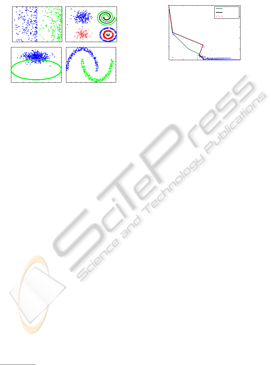
Figure 2: Synthetic datasets.

2.5 Semi-supervised Context

We want to study the evolution of the AUC as the frac-

tion of data which has labels becomes smaller. We be-

gin by applying the clustering algorithms to the com-

plete datasets, as in previous section. However, only

10% of the points are used to compute the ROC curve,

and consequently the AUC. The whole dataset is used

to perform clustering, whereas the AUC is computed

with only a part of the data. This mimics what would

happen in a real situation if only part of the data had

labels available.

This process is done M times, each time using a

different 10% subset of the data for computing the

AUC. This process is run also with 20%, 30%, ... ,

100% of the points used for the AUC computation.

3 EXPERIMENTAL RESULTS

AND DISCUSSION

We consider several synthetic (see ﬁgure 2) and real

datasets, from the UCI machine Learning Reposi-

tory

, to study the robustness of clustering algorithms

using the measure described in the previous section.

We use 7 traditional clustering algorithms: single-link

(SL), average-link (AL), complete-link (CL), Ward-

link (WL), centroid-link (CeL), median-link (MeL)

and k-means (Theodoridis and Koutroumbas, 2009),

and two clustering algorithms based on dissimilarity

increments: SLAGLO (Fred and Leit

ao, 2003) and

SLDID (Aidos and Fred, 2011).

3.1 ROC and Parameter Selection

SLAGLO and SLDID have one parameter that needs

to be set (Fred and Leit

ao, 2003; Aidos and Fred,

http://archive.ics.uci.edu/ml

0 0.2 0.4 0.6 0.8 1

0.2

0.4

0.6

0.8

AvgError

bestrun

VarPart Init

Figure 3: Synthetic dataset with four clusters. Blue dots

correspond to the error values for 100 different initializa-

tions of k-means. AvgError is the ROC curve correspond-

ing to the mean of type I and II errors; bestrun is the ROC

curve for the best run according to the intrinsic criterion of

k-means; VarPart Init is the ROC curve for k-means with a

ﬁxed initialization based on (Su and Dy, 2007).

2011). As described in section 2.3, we use the AUC

to decide the best parameter for each algorithm.

Figure 3 shows the ROC curves for k-means, for

each strategy described in section 2.3. The ﬁgure

shows that the curve based on the mean of type I and

II errors is proper; the other two are not. This curve

also has the lowest AUC. In the following, we plot

the ROC curve of k-means using several initializa-

tions and the mean of the type I and II errors.

3.2 Fully Supervised Case

In this section we study the case described in sec-

tion 2.4. Figure 4 shows the results of applying the

clustering algorithm to the datasets described above.

For brevity, we present plots only for three of the

datasets; we then summarize all the results in table 1.

From table 1 we can see that SLAGLO is more

robust in the synthetic data than other clustering algo-

rithms. However, in real datasets, WL and CeL seem

to be the best algorithms. In some datasets, we get

high values of ε

and ε

for some algorithms (such

as CL and MeL on the cigar dataset) which indicate

that these clustering algorithms are not appropriate for

that dataset. One of the datasets (crabs) is very hard

to tackle for all algorithms.

3.3 Semi-supervised Case

As described in section 2.5, we simulate a semi-

supervised situation to study the advantages of the

AUC as a clustering evaluation criterion. In these ex-

periments we use M = 50 runs.

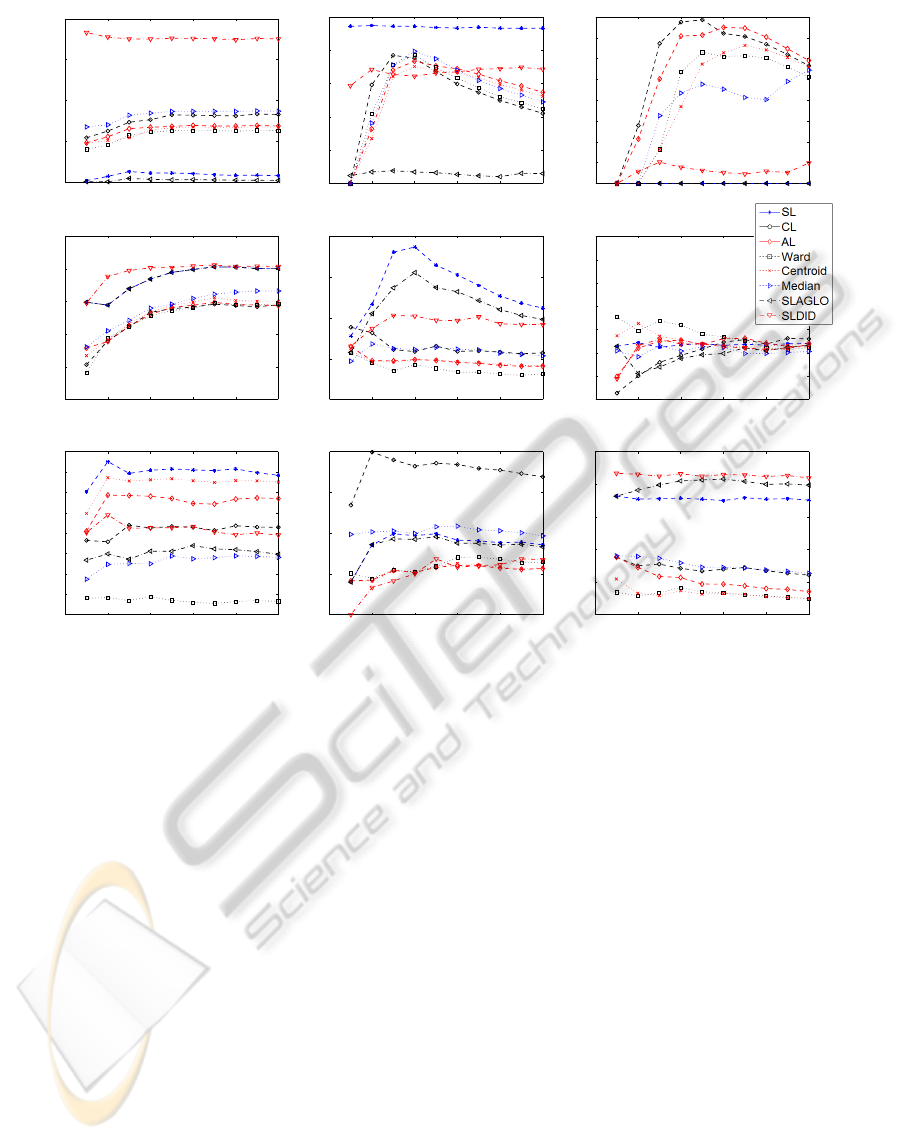
Figure 5 shows the values of the AUC versus the

percentage of points used to compute the AUC. There

is considerably different behavior depending on the

dataset. For example, in the image-1 dataset the AUC

ICPRAM2013-InternationalConferenceonPatternRecognitionApplicationsandMethods

278

0 0.2 0.4 0.6 0.8 1

0.2

0.4

0.6

0.8

breast

0 0.2 0.4 0.6 0.8 1

0.2

0.4

0.6

0.8

iris

0 0.2 0.4 0.6 0.8 1

0.2

0.4

0.6

0.8

barras−c3

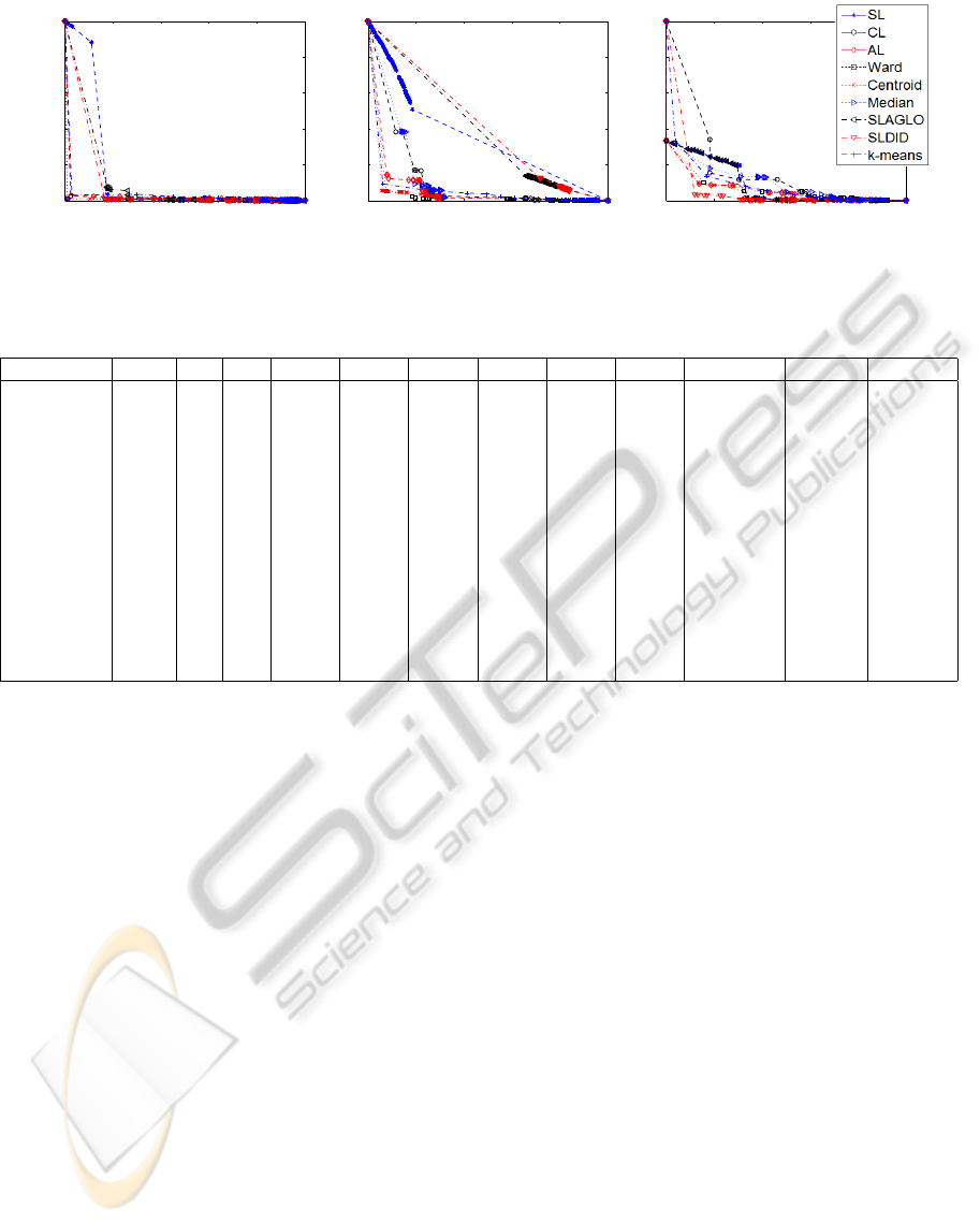
Figure 4: ROC curves for one synthetic datasets and two real datasets.

Table 1: Area under the ROC curve (AUC) when we have access to all labeling of data. Ns is the number of samples, Nf the

number of features and Nc the true number of clusters. The bold numbers are the lowest AUC, which corresponds to the best

clustering algorithm.

Data Ns Nf Nc SL CL AL WL CeL MeL SLAGLO SLDID k-means

barras-c3 400 2 2 0.139 0.025 0.025 0.010 0.010 0.011 0.102 0.087 0.034

image-1 1000 2 7 0.007 0.082 0.068 0.063 0.067 0.087 0.002 0.175 0.074

image-2 1000 2 2 0.467 0.211 0.274 0.224 0.261 0.245 0.030 0.343 0.266

semicircles 500 2 2 0 0.283 0.296 0.256 0.280 0.272 0 0.049 0.320

austra 690 15 2 0.489 0.428 0.472 0.470 0.483 0.486 0.489 0.496 0.320

biomed 194 5 2 0.304 0.279 0.273 0.250 0.280 0.271 0.292 0.408 0.273

breast 683 9 2 0.351 0.121 0.070 0.049 0.049 0.127 0.397 0.419 0.064

chromo 1143 8 24 0.451 0.395 0.394 0.397 0.401 0.416 0.451 0.454 0.403

crabs 200 5 2 0.486 0.501 0.492 0.485 0.498 0.496 0.481 0.480 0.499

derm 366 11 6 0.112 0.057 0.041 0.031 0.041 0.054 0.098 0.092 0.055

ecoli 272 7 3 0.332 0.100 0.072 0.093 0.070 0.162 0.257 0.322 0.095

german 1000 18 2 0.488 0.492 0.485 0.484 0.489 0.481 0.487 0.487 0.487

imox 192 8 4 0.342 0.214 0.285 0.033 0.325 0.140 0.148 0.195 0.134

iris 150 4 3 0.086 0.169 0.057 0.064 0.057 0.097 0.083 0.067 0.089

of all algorithms is roughly constant and does not vary

much with the percentage of labeled points.

In other datasets we see something very different:

in the semicircles and image-2 datasets some methods

have a low AUC for a low percentage of labeled points

which then starts to increase with this percentage.

These two different behaviors illustrate an impor-

tant aspect of the AUC for semi-supervised situations:

this measure can become very low for very small per-

centages of labeled points. In the cases described pre-

viously, this is merely a spurious value, since if we

had more information (more labeled points) we would

ﬁnd out that the AUC is actually higher.

On the other hand, these plots allow us to decide

whether it is worth it to label more data. In general, la-

beling datasets is expensive; for this reason, it is use-

ful to know if labeling only a subset of data will be

enough. One can plot part of the AUC vs. fraction of

labeled points curve using the data which is already

labeled. If this curve is approximately constant, then

it is likely that labeling more data won’t bring much

beneﬁt. If this curve is rising, then it might be worth

considering the extra effort of labeling more data, un-

til one starts seeing convergence in this curve.

There is a further use for these curves. In general,

the best way of knowing whether a partition of the

data is correct is to know the true partition. In some

cases, like in the WL for the imox dataset, the curve

is both constant and has a very low value. If one starts

investing the time and/or money to label, say, 40% of

the data, one can already be quite sure that the clus-

tering provided by WL is a good one, even without

labeling the rest of the data. This is applicable to a

few more algorithm-dataset combinations: WL, AL

and CeL for derm, or SLDID, AL and WL for iris.

If labeling more data is completely infeasible, the

previous reasoning will at least allow researchers to

know whether the results obtained on the partially-

labeled data are reliable or not.

4 CONCLUSIONS

There are several criteria to evaluate the performance

of clustering algorithms. However, those criteria only

evaluate clustering algorithms for a ﬁxed number of

clusters, k. In this paper, we proposed the use of a

ROC curve to study the performance of an algorithm

for several k simultaneously. This allows measuring

how robust a clustering method is to the choice of k.

TheAreaundertheROCCurveasaCriterionforClusteringEvaluation

279

0 20 40 60 80 100

0.05

0.1

0.15

0.2

% of samples

AUC

image−1

0 20 40 60 80 100

0.1

0.2

0.3

0.4

0.5

% of samples

AUC

image−2

0 20 40 60 80 100

0.05

0.1

0.15

0.2

0.25

0.3

0.35

0.4

% of samples

AUC

semicircles

0 20 40 60 80 100

0.25

0.3

0.35

0.4

0.45

0.5

% of samples

AUC

chromo

0 20 40 60 80 100

0.05

0.1

0.15

0.2

% of samples

AUC

derm

0 20 40 60 80 100

0.44

0.46

0.48

0.5

0.52

0.54

0.56

0.58

% of samples

AUC

german

0 20 40 60 80 100

0.05

0.1

0.15

0.2

0.25

0.3

0.35

0.4

% of samples

AUC

imox

0 20 40 60 80 100

0.05

0.1

0.15

0.2

% of samples

AUC

iris

0 20 40 60 80 100

0.1

0.2

0.3

0.4

0.5

% of samples

AUC

breast

Figure 5: Average of AUC over 50 random subsets of data where we use % of samples with labels to obtain the ROC curves.

Moreover, in order to compare the robustness of

different clustering algorithms, we proposed to use

the area under each ROC curve (AUC).

We showed values of the AUC for fully supervised

situations. Perhaps more interestingly, we showed

that this measure can be used in semi-supervised

cases to automatically detect whether labeling more

data would be beneﬁcial, or whether the currently la-

beled data is already enough. This measure also al-

lows us to extrapolate classes from the labeled data to

the unlabeled data, if one can ﬁnd a clustering algo-

rithm which yields low and consistent AUC value for

the labeled portion of the data.

ACKNOWLEDGEMENTS

This work was supported by the Portuguese Founda-

tion for Science and Technology grant PTDC/EIA-

CCO/103230/2008.

REFERENCES

Aidos, H. and Fred, A. (2011). Hierarchical clustering with

high order dissimilarities. In Proc. of Int. Conf. on

Mach. Learning and Data Mining, 280–293.

Bolshakova, N. and Azuaje, F. (2003). Cluster validation

techniques for gene expression data. Signal Process-

ing, 83:825–833.

Bradley, A. P. (1997). The use of the area under the

roc curve in the evaluation of machine learning algo-

rithms. Patt. Recog., 30(7):1145–1159.

Fred, A. and Leit

ao, J. (2003). A new cluster isolation cri-

terion based on dissimilarity increments. IEEE Trans.

on Patt. Anal. and Mach. Intelligence, 25(8):944–958.

Halkidi, M., Batistakis, Y., and Vazirgiannis, M. (2001). On

clustering validation techniques. Journal of Intelligent

Information Systems, 17(2-3):107–145.

Jain, A., Murty, M., and Flynn, P. (1999). Data clustering:

a review. ACM Comp. Surveys, 31(3):264–323.

Su, T. and Dy, J. G. (2007). In search of deterministic

methods for initializing k-means and gaussian mixture

clustering. Intelligent Data Analysis, 11(4):319–338.

Theodoridis, S. and Koutroumbas, K. (2009). Pattern

Recognition. Elsevier Academic Press, 4th edition.

ICPRAM2013-InternationalConferenceonPatternRecognitionApplicationsandMethods

280