Resonant Acoustic Sensor System for the Wireless Monitoring

of Injection Moulding

F. M¨uller

, P. O’Leary

, G. Rath

, C. Kukla

, M. Harker

, T. Lucyshyn

and C. Holzer

Chair of Polymer Processing, Montanuniversitaet Leoben, Otto Gloeckel-Strasse 2, Leoben, Austria

Chair of Automation, Montanuniversitaet Leoben, Leoben, Austria

Industrial Liasion Department, Montanuniversitaet Leoben, Leoben, Austria

Keywords:

Pattern Recognition, Gibbs Error, Discrete Fourier Spectrum, Orthogonal Complement, Covariance Propaga-

tion, Discrete Fourier Transform.

Abstract:

The production of high quality plastic parts requires in-mould sensors to monitor the injection moulding pro-

cess. A novel wireless sensor concept is presented where structure borne sound is used to transmit information

from the inside of an injection mould to the outside surface, eliminating the need for cabling within the mould.

The sound is acquired and analyzed using new algebraic basis function techniques to enable the detection of

temporal occurrence of frequency patterns in the presence of large levels of noise. The temporal occurrence

of the resonators represents the passing melt front. The reduction of spectral leakage is computed by an al-

ternative method using low degree Gram polynomials. The computation of the pattern matching algorithm

yields both the correlation coefﬁcients and their covariances which are used to determine the certainty of the

measurement. The paper presents the used mathematical background as well as real measurements performed

on an injection moulding machine. A test mould was equipped with two different resonant structures. Be-

sides calculating the correlation coefﬁcients the 3σ conﬁdence interval of the coefﬁcients is computed. With

the novel algebraic approach a reliable separation of the two temporal points of occurrence of the resonant

structures was computed.

1 INTRODUCTION

Injection moulding is the most important manufactur-

ing process for plastic parts. In this highly dynamic

process a lot of effort went into the development of the

control algorithms of the injection moulding machine

concerning repeatability (Chen and Turng, 2005; Gi-

boz et al., 2007; Kamal et al., 1984). In contrast

the injection mould is often neglected in terms of

implementing control elements in form of sensors.

There are mainly two types of in-mould sensors that

are common, cavity wall temperature- and pressure-

sensors (Giboz et al., 2007) which always transmit

the measured values by wires. Since wires have some

disadvantages concerning mould design and mainte-

nance effort (Zhang et al., 2005), current research in

the ﬁeld of wireless in-mould sensors presents differ-

ent approaches (Bulst et al., 2001; Gao et al., 2008;

Zhang et al., 2005).

In this paper a different approach is shown where

no active circuitry within the mould is required

(M¨uller et al., 2012). A distinctive structure borne

sound is generated on purpose by a mechanical res-

onator which is excited by the passing melt front.

Hence, the temporal event when the melt front passes

the resonator can be detected. This temporal resolu-

tion of the passing melt front is of special interest for

example for detecting the switch over point (from ﬁll-

ing to holding pressure phase) or for hot runner bal-

ancing (Kazmer et al., 2010; Frey, 2004).

The main contributions of this paper are:

1. A new sensor concept is presented for wireless

monitoring of the ﬁlling of moulds during injec-

tion moulding;

2. Structure borne sound is used to implement wire-

less transmission of information from multiple

positions to a single accelerometer mounted out-

side the mould. This eliminates the need for ca-

bling within the mould, making the mould both

cheaper in construction and simpler to service;

3. The design of a mechanical resonator is combined

with a new signal processing method to enable

the detection of multiple events in the single time

153

Müller F., O’Leary P., Rath G., Kukla C., Harker M., Lucyshyn T. and Holzer C..

Resonant Acoustic Sensor System for the Wireless Monitoring of Injection Moulding.

DOI: 10.5220/0004266301530161

In Proceedings of the 2nd International Conference on Sensor Networks (SENSORNETS-2013), pages 153-161

ISBN: 978-989-8565-45-7

 2013 SCITEPRESS (Science and Technology Publications, Lda.)

varying signal;

4. A new algebraic approach to the implementa-

tion of frequency domain pattern matching is pre-

sented. The new approach yields a numerically

very efﬁcient solution to computing the desired

correlation coefﬁcients. Furthermore and very im-

portant for measurements in an industrial environ-

ment, the new method also yields a method for

estimating the covariance of the correlation coef-

ﬁcients. Consequently, the detection of an event

can be made with a given certainty.

2 PRINCIPLE OF OPERATION

The aim is to develop a system which is capable of de-

tecting when the melt front reaches speciﬁc regions in

a mould, i.e. the detection of discrete temporal events.

Multiple detections should be possible and there is

the further desire not to have any cabling within the

mould. This makes the mould simpler in construc-

tion and easier to service. The principle of operation

is very simple, see Figure 1: The dark portion in the

ﬁgure represents the melt (A) ﬁlling the cavity (B).

When the melt reaches the pin (C) it is depressed and

excites the resonator (D), which injects a characteris-

tic sound into the metal mass of the mould. This por-

tion of the system is purely mechanical. The sound is

acquired using a single accelerometer and analyzed.

Figure 1: Schematic drawing of the principle of operation.

The dark portion (A) represents the melt ﬁlling the cav-

ity (B). When the melt reaches the pin (C) it is depressed

and excited the resonator (D). This portion of the system is

purely mechanical (M¨uller et al., 2012).

The sensor system consists of three main portions:

1. Mechanical resonators, these are purely mechani-

cal devices which exhibit a characteristic damped

oscillatory behaviour. When excited they res-

onate and introduce structure borne sound into the

metallic mass of the mould.

2. A single accelerometer mounted on the outside of

the mould. This accelerometer detects the struc-

tural borne sound from all the mechanical res-

onators.

3. A signal acquisition and processing unit, which

acquires the signal from the accelerometer and

implements a new matrix algebraic approach to

pattern recognition. The system enables the detec-

tion of the time points of excitation of the different

mechanical resonators and with this the detection

of the melt front at the desired points in the mould.

This paper presents the development of the com-

plete detection system.

2.1 Mechanical Resonator

In Figure 2 a rendered section view of a mechanical

resonator is shown. The system consists of: a sprung

movable pin (A and B), and a resonant body (C). The

spring ensures the pin is in the correct position prior to

excitation. When the melt reaches the position in the

mould where the pin is, it accelerates the pin and ex-

cites the resonant body. The pin, spring and resonant

body form a damped resonator which emits a charac-

teristic acoustic signal into the metallic body of the

mould.

Figure 2: Rendered section view of one of the implemented

mechanical resonators. The pin (A) which is pushed by the

melt, the spring (B) which positions the pin and the reso-

nant body (C). This Figure shows the implemented 12[kHz]

resonator (M¨uller et al., 2012).

Two different resonator designs were imple-

mented for test purposes

1. A plate resonator, as shown in Figure 2, with a

primary resonant mode at 12[kHz], and

2. a tongue resonator, not shown, with a primary res-

onant mode at 3.8[kHz].

Both designs use the same mechanical components

(housing, pin and spring), only the resonant body is

exchanged. In this manner different resonant char-

acteristics can be simply implemented. The different

For simplicity in the rest of the paper the two resonators

are identiﬁed by their primary modal frequency.

SENSORNETS2013-2ndInternationalConferenceonSensorNetworks

154

oscillatory characteristics enable the separation of the

events from the different resonators in the signal ac-

quired from one and the same accelerometer.

2.2 Acoustic Detection

A single accelerometer is mounted on the outside

of the mould. It detects the structure borne sounds

from all the resonators. The accelerometer (352A60

from PCB Piezotronics) has a frequency range from

5−60000[Hz] and was sampled

with f

= 120[kHz].

The high frequency range has been chosen to improve

the performance of the system in the presence of sig-

niﬁcant acoustic disturbances associated with the op-

eration of the machine.

The high sampling frequency gives a larger num-

ber of spectral components which can be used in the

pattern recognition to detect the desired oscillations.

The resonators have multiple harmonics which yield

multiple correlated components in the frequency do-

main. However, the wider range of noise acquired

with the higher sampling frequency is uncorrelated.

Consequently, a better signal to noise ratio can be

achievedin this manner. The signal acquisition is syn-

chronized with the start of the injection process.

2.3 Signal Processing

The aim of the signal processing is to implement

optimal detectors, optimal in terms of noise perfor-

mance, for the characteristic oscillations of the res-

onators. Due to the complex mechanical form and

internal reﬂections within the mould, the signals from

the resonators are not fully orthogonal. Consequently

classical correlation detectors (Fano, 1951) will not

function optimally. This paper presents a new al-

gebraic approach to signature recognition, which is

numerically efﬁcient, while maintaining the advan-

tages of full spectrum pattern matching. In addition to

the matching of the pattern the new method also im-

plements the covariance propagation, which in turn

yields a conﬁdence interval. Consequently, the cer-

tainty of the measurement is also determined. The

details are presented in the following section.

3 MATHEMATICAL

FRAMEWORK

In this paper a new algebraic implementation of a fre-

quency domain signature matching is implemented.

For test purposes the signal was acquired using a data

acquisition box from National Instruments (USB-6366).

There are two steps involved in signature matching:

1. Signature identiﬁcation, i.e. identifying the op-

timal frequency domain signatures for each res-

onator. This task is performed a-priori to the mea-

surement and can be considered as a calibration of

the system.

2. Signature matching, which is formulated as a lin-

ear matrix algebraic computation. This method is

numerically efﬁcient and the covariance propaga-

tion for the linear operator can be computed.

Before proceeding to these two steps it is neces-

sary to introduce a matrix algebraic approach to com-

puting a discrete Fourier transform (DFT) and a new

method for reducing the effects of the Gibbs phe-

nomena. In most common literature on digital signal

processing, e.g., (Press et al., 2002; Oppenheim and

Schafer, 1989), the computation of the DFT is formu-

lated as,

s(k) =

N−1

∑

n=0

y(n)e

− j2πkn/N

(1)

whereby, y(n) is the n

sample of the input signal, N

is the total number of samples available, and k deﬁnes

the discrete frequency f

= (2πkn/N) f

, with respect

to the sampling frequency f

. Given N input samples

there are N components in the discrete Fourier spec-

trum. Computing the discrete Fourier series is most

commonly called the discrete Fourier transform and

is most commonly implemented using the fast Fourier

transform (FFT) algorithm. The FFT and DFT are

functionally identical, the FFT is simply a numeri-

cally more efﬁcient method of performing the com-

putation.

The computation of the DFT can also be formu-

lated as a matrix

operation. The discrete Fourier ba-

sis functions f(k),

f(k) , e

− j2πkn/N

, (2)

can be concatenated forming the columns of a matrix

F, such that

F ,



f(0),... , f(N − 1)



. (3)

Now given a vector y of N input samples, the com-

plete spectrum s, a vector, of the signal y is computed

as,

s = F y. (4)

Computing the discrete Fourier spectrum in this man-

ner is signiﬁcantly less efﬁcient than computing an

A brief note on nomenclature: matrices are indicated

by sanserif capital letters, e.g. H, and vectors by sanserif

lowercase letters, e.g. y.

The matrix F can be generated in MATLAB using the

code, F = dftmtx(N)

′

ResonantAcousticSensorSystemfortheWirelessMonitoringofInjectionMoulding

155

FFT if ﬁnally all spectral components are required.

However, as shall be seen, given the need to only

identify a low number of signatures the method offers

signiﬁcant advantages, both with respect to numerical

efﬁciency as also in estimating conﬁdence intervals.

Prior to computing the spectrum it is necessary to

take measures so as to limit the errors associated with

the Gibbs phenomena. The classical approach is to

use windowing (Press et al., 2002; Lindquist, 1988),

however, a new method based on polynomial approx-

imation was introduced recently, see (O’Leary and

Harker, 2011) for derivations and exact nature of the

computation. The signal is projected onto the orthog-

onal complement of a set of Gram polynomial basis

functions of low degree. The Gram polynomial ba-

sis functions up to degree d are also used to form the

columns of a matrix G

, the projection P onto the or-

thogonal complement can be computed as,

P = I − G

, (5)

where I is the unit matrix.

The spectrum with reduced spectral leakage is

now computed as,

s = F



I − G



y. (6)

It should be noted that, H , F



I − G



is once

again a matrix. In this manner reducing the Gibbs

effect has added no additional numerical complexity,

since H can be computed a-priori.

3.1 Signature Identiﬁcation

The calibration procedure takes advantage of super-

position, in the assumption that the noise of the ma-

chine and the sound from the resonator can be re-

garded as additive signals. The i

resonator alone is

artiﬁcially activated while the machine is not running.

The signal from the accelerometer is acquired and the

corresponding spectrum is computed,

= H y. (7)

This procedure is repeated for each resonator yield-

ing a set of n initial spectral signatures one for each

resonator. Unfortunately, due to the complicated me-

chanical forms and internal acoustic reﬂections within

the form these vectors are not fully orthogonal.

The orthogonality of the signatures is achieved by

projecting them onto their mutual orthogonal comple-

ments. Given n signatures this is computed as,

ˆs

(

I −

∑

∀ k ∈ [1. .. n],k 6= i. (8)

To support understanding it is helpful to formulate

this computation for two signatures,

ˆs

= s

− s



I − s



(9)

ˆs

= s

− s



I − s



. (10)

This computation yields a set of n orthogonalized sig-

natures ˆs

, which are complex vectors each of length

N. These are then used in the signature matching pro-

cess. The matrix of signatures S is formed by con-

catenating the individual orthogonalized vectors and

dividing them by their norm,

S =

ˆs

|ˆs

,.. .,

ˆs

|ˆs

. (11)

In this manner the matrix S has a unitary norm. Con-

sequently, S

, which is discussed next, has also a uni-

tary norm.

The orthogonalization process described by Equa-

tions 9 and 10 have worked well with the sensors used

in the experiment presented in this paper. However,

other experiments suggest that a diagonalisation of

the matrix of signatures, using singular value decom-

position, yields an even better separation of the sig-

nals with a lower cross sensitivity. This issue, how-

ever, is still the subject of further investigation.

3.2 Signature Matching

To support understanding it is helpful to take a more

fundamental look at the nature of the system and the

computation being performed. The excitation of the

pin can be approximated as a dirac pulse, in this case

the signatures correspond to the impulse response of

the resonators. For simplicity the orthogonalization

process is not considered now. The impulse response

corresponds to the ﬁrst eigenfunction of the differ-

ential equation describing the dynamics of the res-

onator. Given a measurement of the resonator’s re-

sponse, with the addition of noise, the task is to per-

form de-convolution of the measured signal with the

response of the differential equation. This is funda-

mentally an inverse problem. In a lose sense it is

equivalent to inversion of the stochastic differential

equation for the system.

An algebraic approach to the computation has

been chosen since the Moore-Penrose pseudo-

inverse (Golub and Van Loan, 1996) provides a least

square approximation for the inversion of a rectangu-

lar matrix,





−1

, (12)

which ensures,

S = I. (13)

Computing S

is akin to inverting the eigenfunctions

contained in S which describe the differential equa-

tions of the resonators.

SENSORNETS2013-2ndInternationalConferenceonSensorNetworks

156

The input signal is continually acquired and a sub-

set of N values are selected to form the vector y. The

spectrum of the signal is computed as shown in Equa-

tion 6,

= H y. (14)

This is called the temporal varying signature s

. It

should be noted that it may contain zero or any num-

ber of the sought events. The correlation coefﬁcient

to the n signatures is computed as,

c = S

= S

Hy, (15)

where c is an n element column vector

5,6

. The ma-

trix L can now be deﬁned as L , S

H, this is of size

N × n, in the test case here n = 2 and N = 600. This

matrix is computed a-priori to measurement; conse-

quently computing the correlation coefﬁcients at run-

time is numerically very efﬁcient and can be written

as,

c = L y. (16)

The computation is repeated p samples later.

Computation in this manner is very closely related

to the short-time Fourier transform (STFT). For those

more familiar with classical digital signal processing:

the columns of L can be considered to be the coef-

ﬁcients of a ﬁnite impulse response (FIR) ﬁlter (Op-

penheim and Schafer, 1989), with a decimation factor

p. Consequently, there is a bank of n FIR ﬁlters given

n resonators.

3.3 Covariance Propagation

The covariance (Brandt, 1998) for a vector is deﬁned

as,

, {c − E(c)} {c − E(c)}

. (17)

Now substituting the relationship c = Ly, yields,

= {Ly − L E(y)} {Ly − L E(y)}

, (18)

and factoring out L,

= L {y − E(y)} {y − E(y)}

. (19)

To facilitate numerical efﬁciency the correlation coefﬁ-

cients can be computed as,

c = S

abs(Hy).

The norm of



is 1 and the norm of |H| = 1− 2/n, in the

application n = 600, therefor |H| ≈ 1. Consequently, this

numerical simpliﬁcation does not change the norm of the

result.

Ideally this computation should yield only real values

for c; however, due to numerical errors small imaginary

components may remain. For this reason, it is suggested

to take only the real portion, i.e., R (c).

By deﬁnition Λ

, {y − E(y)} {y − E(y)}

, conse-

quently,

= L Λ

. (20)

If we can regard the input noise to the system as inde-

pendent identically distributed (i.i.d.) Gaussian errors

with standard deviation σ, the covariance of the input

is given by,

= σ

I, (21)

and consequently,

= σ

. (22)

In this manner we also have an estimator for the co-

variance of the correlation coefﬁcients. This is one of

the major advantages of using an algebraic approach

to solve this problem. No other computation method

would yield the covariance estimates in such a simple

manner.

3.4 Decision Process

Given the vector of correlation coefﬁcients c and the

associated covariance matrix Λ

: a decision with a de-

sired conﬁdence interval can be made.

There is a delay of N samples for the ﬁrst deci-

sion and then a decision follows every P samples. The

group delay for an FIR ﬁlter with N symmetric coefﬁ-

cients is t

= N/(2 f

), for example in this application

with f

= 120[kHz] and a signature length of N = 600

there is a decision delay of t

= 2.5[ms] and a new de-

cision is available every t

= 0.42[ms].

4 EXPERIMENTAL SETUP

AND RESULTS

The experiments were performed on an Arburg in-

jection moulding machine (470A-1000) with a Poly-

Propylen (C7069-100NA) from Dow. The injection

speed was set to 60[cm

−1

]. The diameter of the

injection screw is 40[mm]. For the measurements a

test mould was built. The mould consists of two sym-

metrical cavities which are gated by a hot runner sys-

tem (Johannaber and Michaeli, 2004). The hot runner

system is equipped with an electromagnetic valvegate

control. Two test resonators with different designs

were implemented and installed in the test mould.

Figure 3 shows a picture of the clamped mould in

the injection moulding machine. The mould is shown

in the opened position. During processing the mould

is closed and charged with a clamping force of ap-

proximately 900[kN]. The two symmetric cavities are

indicated by A and B. The accelerometer in the pic-

ture is marked with C, which is mounted on the out-

side surface of the mould.

ResonantAcousticSensorSystemfortheWirelessMonitoringofInjectionMoulding

157

Figure 3: Picture of the mould clamped in the injection

moulding machine. The mould is shown in opened posi-

tion. During the production process the mould is closed and

charged with a clamping force of approximately 900[kN].

A and B indicate the two symmetrical cavities; C marks the

position of the accelerometer mounted on the outside sur-

face of the mould.

4.1 Experimental Signature

Identiﬁcation

The machine is not running during identiﬁcation of

the signatures. This reduces the spurious presence

of noise during this process. Since there are two

resonators implemented in the mould n = 2. As

previously mentioned a sampling frequency of f

120[kHz] was used. Both resonators were excited in-

dependently and their time response was measured.

In Figure 4 the time response as a function of time

for both resonators is shown. It is important to note

that the resonator nominally designed for 3.8[kHz]

has many overtones which lead to higher frequency

components than the 12[kHz] resonator.

The sampled data was segmented into packets

containing N = 600 samples. Each packet is projected

onto the orthogonal complement of a Gram polyno-

mial G

of degree d = 1 prior to computing the cor-

responding discrete Fourier spectrum, this suppresses

signiﬁcant portions of the spectral leakage. The ob-

tained signatures are not fully orthogonal due to the

complex mechanical form of the mould as well as

acoustic reﬂections inside it.

Therefore the two signatures are then orthogonal-

ized according to Equations 9 and 10. The result-

ing orthogonalized signatures are shown in Figure 5.

Since the magnitude spectrum of a real signal is sym-

metric, only the ﬁrst N/2, i.e., 300 values are shown.

From the spectrum it gets clear, that there are just

signiﬁcant frequency components up to approximatly

20[kHz]. With a given sampling rate of 120[kHz]

0 1 2 3 4 5

−0.2

0.2

(t)

0 1 2 3 4 5

−0.5

0.5

(t)

Time [m s]

Figure 4: Top: the time response of the 12[kHz] resonator.

Bottom: the time response of the 3.8[kHz] resonator. It is

important to note that the resonator nominally designed for

3.8[kHz] has many overtones. This lead to higher frequency

components. Each of the time signatures consists of 600

samples. The shown results were measured independently

and are not shown synchronized.

this means that just the ﬁrst 50 values of the spec-

trum are required for event identiﬁcation. Since the

noise is distributed over 600 values of the spectrum

and just 50 of them are needed, this corresponds to

an implicit regularization. This yields a noise gain of

50/600.

The two orthogonalized signatures, ˆs

(ω) and

ˆs

(ω), are used during further processing.

0 10 20 30

0.2

0.4

ˆs

(ω)

0 10 20 30

0.2

0.4

ˆs

(ω)

Frequency [kHz]

Figure 5: Top: the spectrum of the impulse response of the

12[kHz] resonator. Bottom: the spectrum of the impulse re-

sponse of the 3.8[kHz] resonator. Here, as in Figure 4, the

higher frequency components associated with the harmon-

ics of the 3.8[kHz] are visible in the spectrum. Note there

are only signiﬁcant magnitudes in the range up to approxi-

mately 20[kHz]. Given the sampling frequency of 120[kHz]

this means only 50 components are required to identify the

events. This corresponds to an implicit regularization, the

noise is distributed over 600 of which only 50 are used. This

yields a noise gain of g

50/600.

4.2 Experimental Signature Matching

During signature matching the machine is running

and the process is subject to large levels of spurious

noise emitted from the mechanisms of the injection

SENSORNETS2013-2ndInternationalConferenceonSensorNetworks

158

moulding machine and process. At the beginning of

the injection moulding cycle the valves are opened

which results in a large excitation of the time signal

at the beginning of the measurement (see beginning

of Figure 6). Despite having a fully symmetrical ﬂow

channel system there will be an unbalanced ﬁlling

of the cavities, having tolerances and inhomogeneous

temperature distributions (Johannaber and Michaeli,

2004). To compensate the unbalanced ﬁlling and en-

sure simultaneous ﬁlling of both cavities the valves

are opened consecutively whereby the opening delay

is controlled by a closed loop controller. In each of

the cavities a resonator is implemented, the left cav-

ity with the 12[kHz] resonator, the right one with the

3.8[kHz] resonator.

The measurements were synchronized to the start

of the injection moulding process. The data acquisi-

tion box records the accelerometer channels for a du-

ration of 10[s]. The ﬁrst 2[s] of the recorded signal

are shown in Figure 6. It can be seen that the signal

is perturbed with large levels of noise. It is assumed

that the noise is distributed as i.i.d. Gaussain noise

with σ = 1.6e−4.

0 0.5 1 1.5 2

−1

−0.5

0.5

Time [s]

y(t) [V]

Figure 6: First 2[s] of recorded accelerometer signal shown

in time domain. The signal is perturbed with noise over the

whole measurement. The noise is assumed as i.i.d Gaussian

noise, σ = 1.6e−4. The searched resonators both appear in

the time domain at approximately 1.1[s] after start of the

ﬁlling phase. The exact time point is estimated with the

correlation coefﬁcient computation.

To support understanding, the short time Fourier

transform (Spectrogram) of the signal is computed

and shown in Figure 7. Thereby just the period

where the frequency patterns are expected is shown

in the spectrogram. At approximately 1.06[s] the

12[kHz] resonator is found, at approximately 1.08[s]

the 3.8[kHz] resonator. The temporal positions of the

events were identiﬁed using signature matching, i.e.

via the correlation coefﬁcients which are discussed

later. This visualization is not required during normal

operation.

The correlation coefﬁcients were computed as

proposed in Equation 15 and are shown with a

Frequency [kHz]

Time [s]

STFT

3.8 kHz12 kHz

1.02 1.04 1.06 1.08 1.1

Figure 7: Magnitude spectrogram of the accelerometer sig-

nal, in addition the time points when the resonator events

occurred are shown, for both the 3.8[kHz] and 12[kHz] res-

onators. The temporal positions of the events were identi-

ﬁed using the signature matching, i.e. via the correlation

coefﬁcients.

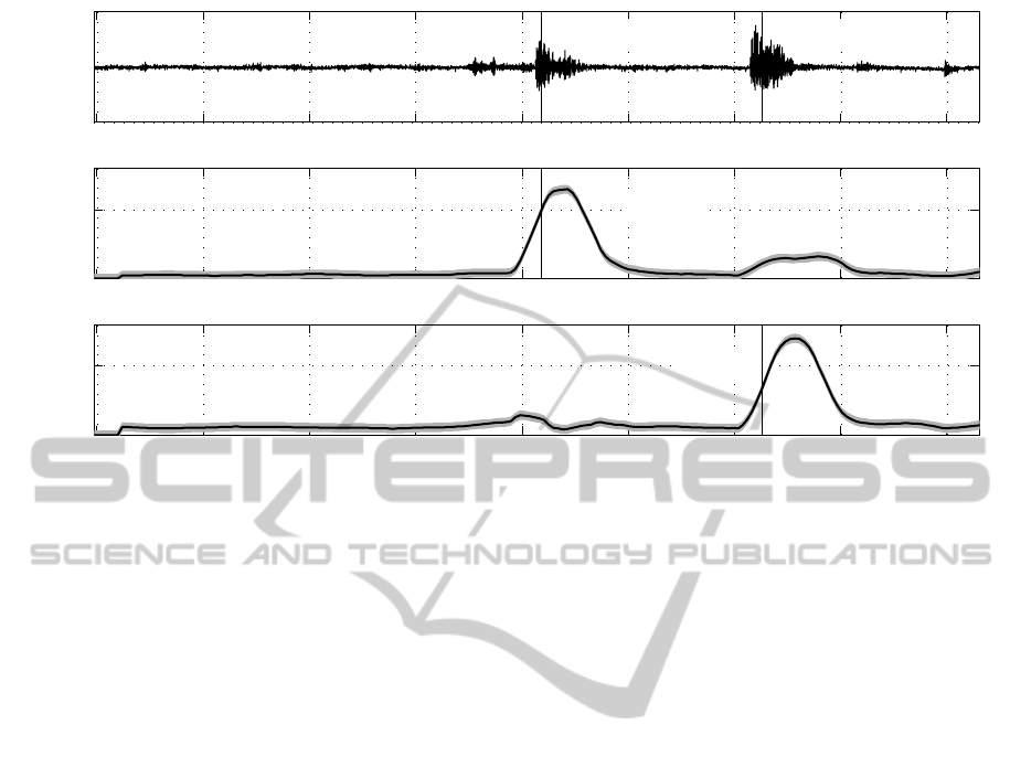
3σ (99.73%) conﬁdence interval in Figure 8 (mid-

dle: c

(t) for the 12[kHz] resonator; bottom: c

(t) for

the 3.8[kHz] resonator). The top diagram shows the

recorded data y(t) in the time domain.

Regarding c

(t), the solid black line indicates the

computed coefﬁcients. In addition, a gray band indi-

cates the 3σ (99.73%) conﬁdence interval. The con-

ﬁdence interval is calculated by the covariance matrix

, which is computed after Equation 22 as,



0.91630 0.79795

0.79795 0.91630



. (23)

Since the matrix Λ

is symmetric and has the identi-

cal values in the diagonal, a symmetric 3σ(99.73%)

conﬁdence interval for both components, i.e. c

(t)

and c

(t), is calculated as ±2.8.

The value of c

, corresponding to the 12[kHz] res-

onator, stays at a low level up to 1.059[s] where a

peak appears. At 1.061[s] a black vertical line indi-

cates the detection of the 3.8[kHz] resonant structure.

The detection is computed with descriptive statistics

(Haase, 2002).

The second correlation coefﬁcient c

, correspond-

ing to the 3.8[kHz] resonator, shows a peak starting at

1.080[s]. The temporal occurrence event was recog-

nized at 1.082[s].

For both detection events a cross correlation can

be observed. Since the cross correlations are small

compared to the peak values of c a reliable separation

of both events can be ensured.

Figure 8 (top) shows the time domain signal y(t)

of the recorded accelerometer data with indicated

events for both resonant structures. It has to be noted

Mainly the calculation of the standard deviation and the

skewness as well as a probability density function are used

for computing the detection.

ResonantAcousticSensorSystemfortheWirelessMonitoringofInjectionMoulding

159

1.02 1.03 1.04 1.05 1.06 1.07 1.08 1.09 1.1

−0.5

0.5

y(t) [V]

3.8 kHz12 kHz

1.02 1.03 1.04 1.05 1.06 1.07 1.08 1.09 1.1

12 kHz

(t)

1.02 1.03 1.04 1.05 1.06 1.07 1.08 1.09 1.1

3.8 kHz

Time [s]

(t)

Figure 8: top: amplitude signal y(t) from the accelerometer, the time points for the identiﬁcation of the two events are also

shown. Middle: the black line shows the correlation coefﬁcient c

(t) for the 12[kHz] resonator as a function of time, the

gray region around the line is the 3σ, i.e., 99.73%, conﬁdence interval for the correlation. Bottom: the black line shows the

correlation coefﬁcient c

(t) for the 3.8[kHz] resonator as a function of time, the gray region around the line is the 3σ, i.e.,

99.73%, conﬁdence interval for the correlation. Some cross sensitivity of the correlations can be observed. However, they are

sufﬁciently small to ensure a reliable separation of the two events.

that the coefﬁcients c both start rising slightly before

the deﬂection of the time domain signal. This lead

from the fact that the signal is segmented into pack-

ets. These packets are evaluated at their center point.

In terms of the injection moulding process the

temporal detection point of the resonant structures in-

dicate the passing melt front.

5 CONCLUSIONS

In this paper a novel wireless in-mould sensor for in-

jection moulding was presented. The sensor is ca-

pable to detect the melt front at certain predeﬁned

positions in the cavity. The data transmission is ob-

tained by the generation of distinctive sound which

is detected by an outside mould surface mounted ac-

celerometer. To separate multiple implemented sen-

sors a frequency pattern search is performed using a

new linear algebraic approach. This method yields a

numerically efﬁcient approach for computing the cor-

relation coefﬁcients. In addition, the covariance prop-

agation can be estimated which consequently yields

the computation of a conﬁdence interval of the esti-

mated coefﬁcients.

The proposed sensor system and the signal pro-

cessing were tested on an injection moulding ma-

chine. In the mould, two different resonant structures

were implemented. First the process of signature

identiﬁcation was described. The obtained orthogo-

nalized signatures were used for the pattern match-

ing process. Injection moulding cycles were recorded

with an outside mounted accelerometer. The recorded

signal contains the sound of the resonators which is

superposed with large levels of noise from the ma-

chine, the mould and auxiliary units. However, the

described frequency domain pattern matching algo-

rithm was able to ﬁnd both temporal points when the

resonant structures were excited. The detection of the

resonant structures corresponds to the detection of the

temporal moment of the passing melt front. In addi-

tion, the 3σ conﬁdence interval of the computed cor-

relation coefﬁcients was shown.

The process of orthogonalization of the signatures

yields space for further investigation with respect to

perturbation analysis, i.e. achieving optimal sensitiv-

ity for noise.

REFERENCES

Brandt, S. (1998). Data Analysis: Statistical and Computa-

tional Methods for Scientists and Engineers. Springer,

Berlin, 3rd edition.

Bulst, W.-E., Fischerauer, G., and Reindl, L. (2001). State

of the art in wireless sensing with surface acoustic

SENSORNETS2013-2ndInternationalConferenceonSensorNetworks

160

waves. IEEE Transactions on Industrial Electronics,

48(2):265–271.

Chen, Z. and Turng, L.-S. (2005). A review of current

developments in process and quality control for in-

jection molding. Advances in Polymer Technology,

24(3):165–182.

Fano, R. (1951). Signal-to-noise Ratio in Correlation

Detectors. Technical report (Massachusetts Institute

of Technology. Research Laboratory of Electronics).

Massachusetts Institute of Technology, Research Lab-

oratory of Electronics.

Frey, J. (2004). Method for automatically balancing the vol-

umetric ﬁlling of cavities. US Patent 2004/0113303

A1.

Gao, R., Fan, Z., and Kazmer, D. (2008). Injection mold-

ing process monitoring using a self-energized dual-

parameter sensor. CIRP Annals - Manufacturing Tech-

nology, 57(1):389–393.

Giboz, J., Copponnex, T., and M´el´e, P. (2007). Microin-

jection molding of thermoplastic polymers: a review.

Journal of Micromechanics and Microengineering,

17(6):96–109.

Golub, G. and Van Loan, C. (1996). Matrix Computations.

The Johns Hopkins University Press, Baltimore, 3

edition.

Haase, S. (2002). Spectral and statistical methods for vi-

bration analysis in steel rolling. PhD Thesis Monta-

nuniversitaet Leoben.

Johannaber, F. and Michaeli, W. (2004). Handbuch

Spritzgiessen. Hanser, M¨unchen, 2nd edition.

Kamal, M. R., Patterson, W. I., Fara, D. A., and Haber, A.

(1984). A study in injection molding dynamics. Poly-

mer Engineering and Science, 24(9):686–691.

Kazmer, D. O., Velusamy, S., Westerdale, S., Johnston, S.,

and Gao, R. X. (2010). A comparison of seven ﬁlling

to packing switchover methods for injection molding.

Polymer Engineering & Science, 50(10):2031–2043.

Lindquist, C. S. (1988). Adaptive and Digital Signal Pro-

cessing with Digital Filtering Applications. Steward

& Sons.

M¨uller, F., Rath, G., Lucyshyn, T., Kukla, C., Burgsteiner,

M., and Holzer, C. (2012). Presentation of a novel

sensor based on acoustic emission in injection mold-

ing. Journal of Applied Polymer Science. In Press.

O’Leary, P. and Harker, M. (2011). Polynomial approxima-

tion: An alternative to windowing in fourier analysis.

IEEE Proceedings of I2MTC 2011.

Oppenheim, A. and Schafer, R. (1989). Discrete-Time Sig-

nal Processing. Prentice-Hall, Englewood Cliffs, NJ.

Press, W. H., Teukolsky, S. A., Vetterling, W. T., and Flan-

nery, B. P. (2002). Numerical Recipes in C++: The

Art of Scientiﬁc Computing. Cambridge University

Press.

Zhang, L., Theurer, C. B., Gao, R. X., and Kazmer, D. O.

(2005). Design of ultrasonic transmitters with de-

ﬁned frequency characteristics for wireless pressure

sensing in injection molding. IEEE Transactions

on Ultrasonics Ferroelectrics and Frequency Control,

52(8):1360–1371.

ResonantAcousticSensorSystemfortheWirelessMonitoringofInjectionMoulding

161